Calibrating the models
The simulation models in SimGrid have been object of thorough validation/invalidation campaigns, but the default values may not be appropriate for simulating a particular system.
They are configured
through parameters from the XML platform description file and parameters passed via
–cfg=Item:Value command-line arguments. A simulator may also include any number of custom model
parameters that are used to instantiate particular simulated activities (e.g., a simulator developed with the S4U API
typically defines volumes of computation, communication, and time to pass to methods such as execute(), put(), or sleep_for()). Regardless of the potential accuracy of the simulation models, if they are
instantiated with unrealistic parameter values, then the simulation will be inaccurate.
Given the above, an integral and crucial part of simulation-driven research is simulation calibration: the process by which one picks simulation parameter values based on observed real-world executions so that simulated executions have high accuracy. We then say that a simulator is “calibrated”. Once a simulator is calibrated for a real-world system, it can be used to simulate that system accurately. But it can also be used to simulate different but structurally similar systems (e.g., different scales, different basic hardware characteristics, different application workloads) with high confidence.
Research conclusions derived from simulation results obtained with an uncalibrated simulator are questionable in terms of their relevance for real-world systems. Unfortunately, because simulation calibration is often a painstaking process, is it often not performed sufficiently thoroughly (or at all!). We strongly urge SimGrid users to perform simulation calibration. Here is an example of a research publication in which the authors have calibrated their (SimGrid) simulators: https://hal.inria.fr/hal-01523608
MPI Network calibration
This tutorial demonstrates how to properly calibrate SimGrid to reflect the performance of MPI operations in a Grid’5000 cluster. However, the same approach can be performed to calibrate any other environment.
This tutorial is the result of the effort from many people along the years. Specially, it is based on Tom Cornebize’s Phd thesis (https://tel.archives-ouvertes.fr/tel-03328956).
You can execute the notebook network_calibration_tutorial.ipynb) by yourself using the docker image
available at: Dockerfile. For that, run the
following commands in the tutorial folder inside SimGrid’s code source (docs/source/tuto_network_calibration):
docker build -t tuto_network .
docker run -p 8888:8888 tuto_network
Please also refer to https://framagit.org/simgrid/platform-calibration/ for more complete information.
0. Introduction
Performing a realistic simulation is hard and therefore the correct SimGrid calibration requires some work.
We briefly present these steps here and detail some of them later. Please, refer to the different links and the original notebook for more details.
Execution of tests in a real platform
Executing the calibration code in a real platform to obtain the raw data to be analyzed and inject in SimGrid.
MPI Async/Sync modes: Identifying threshold
Identify the threshold of the asynchronous and synchronous mode of MPI.
Segmentation
Identify the semantic breakpoints of each MPI operation.
Clustering
Aggregating the points inside each segment to create noise models.
In this tutorial, we propose 2 alternatives to automatically do the clustering: ckmeans.1d.dp and dhist. You must choose one, test and maybe adapt it manually depending on your platform.
Description of the platform in SimGrid
Writing your platform file using the models created by this notebook.
SimGrid execution and comparison
Re-executing the calibration code in SimGrid and comparing the simulation and real world.
This tutorial focuses on steps 3 to 6. For other steps, please see the available links.
1. Execution of tests in a real platform
The first step is running tests in a real platform to obtain the data to be used in the calibration.
The platform-calibration project provides a tool to run MPI experiments. In a few words, the tool will run a bunch of MPI operations in the nodes to gather their performance. In this tutorial, we are interested in 4 measures related to network operations:
MPI_Send: measures the time spent in blocking MPI_Send command.
MPI_Isend: same for non-blocking MPI_Isend command.
MPI_Recv: time spent in MPI_Recv.
Ping-pong: measures the elapsed time to perform a MPI_Send followed by a MPI_Recv.
The first 3 tests (MPI_Send, MPI_Isend and MPI_Recv) are used to calibrate the SMPI options (smpi/os, smpi/or, smpi/ois) while the Ping-pong is used for network calibration (network/latency-factor and network/bandwidth-factor).
For more detail about this step, please refer to: https://framagit.org/simgrid/platform-calibration
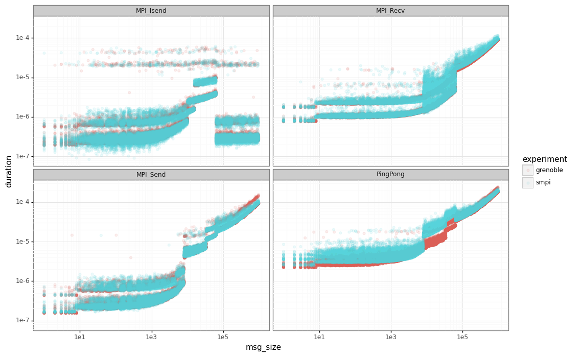
The result of this phase can be seen in the figure below. These are the results for the calibration on Grid’5000 dahu cluster at Grenoble/France.
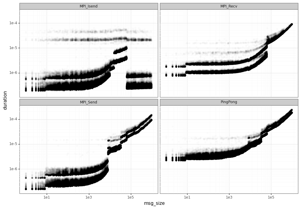
We can see a huge variability in the measured elapsed time for each MPI operation, specially:
Performance leaps: at some points, MPI changes its operation mode and the duration can increase drastically. This is mainly due to the different implementation of the MPI.
Noise/variability: for a same message size, we have different elapsed times, forming the horizontal lines you can see in the figure.
In order to do a correct simulation, we must be able to identify and model these different phenomena.
2. MPI Async/Sync modes: Identifying threshold
MPI communications can operate in different modes (asynchronous/synchronous), depending on the message size of your communication. In asynchronous mode, the MPI_Send will return immediately while in synchronous it’ll wait for respective MPI_Recv starts before returning. See Section 2.2 SimGrid/SMPI for more details.
The first step is identifying the message size from which MPI starts operating in synchronous mode. This is important to determine which dataset to use in further tests (individual MPI_Send/MPI_Recv or PingPong operations).
In this example, we set the threshold to 63305, because it’s the data available in our tests and matches the output of the segmentation tool.
However the real threshold for this platform is 64000. To be able to identify it, another study would be necessary and the adjustment of the breakpoints needs to be made. We refer to the Section 5.3.2 Finding semantic breakpoints for more details.
3. Segmentation
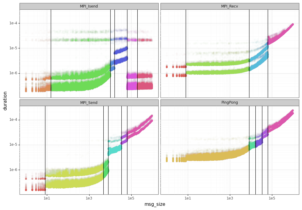
The objective of the segmentation phase is identify the performance leaps in MPI operations. The first step for segmentation is removing the noise by averaging the duration for each message size.
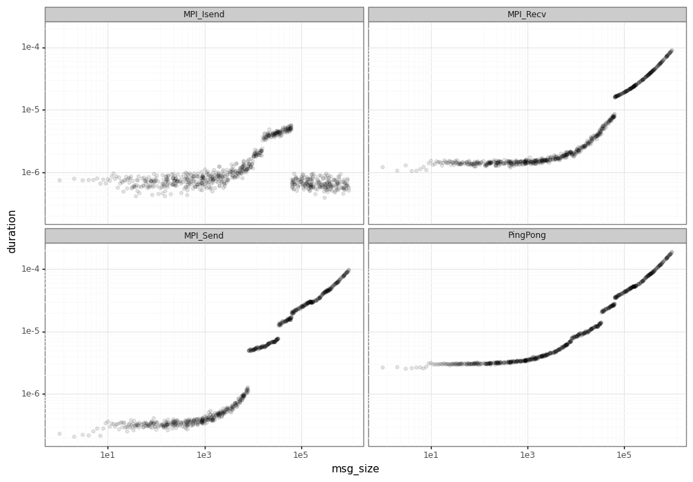
Visually, you can already identify some of the segments (e.g. around 1e5 for MPI_Isend).
However, we use a tool pycewise that makes this job and finds the correct vertical lines which divide each segment.
We present here a summarized version of the results for MPI_Send and Ping-Pong operations. For detailed version, please see “Segmentation” section in network_calibration_tutorial.ipynb.
MPI_Send
| min_x | max_x | intercept | coefficient | |
|---|---|---|---|---|
| 0 | -inf | 8.0 | 2.064276e-07 | 6.785879e-09 |
| 1 | 8.0 | 4778.0 | 3.126291e-07 | 7.794590e-11 |
| 2 | 4778.0 | 8133.0 | 7.346840e-40 | 1.458088e-10 |
| 3 | 8133.0 | 33956.0 | 4.052195e-06 | 1.042737e-10 |
| 4 | 33956.0 | 63305.0 | 8.556209e-06 | 1.262608e-10 |
This is the example of the pycewise’s output for MPI_Send operation. Each line represents one segment which is characterized by:
interval (min_x, max_x): the message size interval for this segment
intercept: output of the linear model of this segment
coefficient: output of the linear model of this segment
The average duration of each segment is characterized by the formula: \(coefficient*msg\_size + intercept\).
Ping-pong
In the ping-pong case, we are interested only in the synchronous mode, so we keep the segments with message size greater than 65503.
| min_x | max_x | intercept | coefficient | |
|---|---|---|---|---|
| 4 | 63305.0 | inf | 0.000026 | 1.621952e-10 |
Setting the base bandwidth and latency for our platform
We use the ping-pong results to estimate the bandwidth and latency for our dahu cluster. These values are passed to SimGrid in the JSON files and are used later to calculate network factors.
To obtain similar timing in SimGrid simulations, your platform must use these values when describing the links.
In this case, the hosts in dahu are interconnected through a single link with this bandwidth and latency.
bandwidth_base = (1.0/reg_pingpong_df.iloc[0]["coefficient"])*2.0
latency_base = reg_pingpong_df.iloc[0]['intercept']/2.0
print("Bandwidth: %e" % bandwidth_base)
print("Latency: %e" % latency_base)
Bandwidth: 1.233082e+10
Latency: 1.292490e-05
3.1. Segmentation results
The figure below presents the results of the segmentation phase for the dahu calibration.
At this phase, you may need to adjust the segments and select those to keep. You can for example do the union of the different segments for each MPI operation to keep them uniform.
For simplicity, we do nothing in this tutorial.
The linear models are sufficient to emulate the average duration of each operation.
However, you may be interested in a more realistic model capable of generating the noise and variability for each message size.
For that, it’s necessary the clustering phase to create specific models for the noise inside each segment.
4. Clustering
We present 2 tool options for creating the noise models for MPI communications: ckmeans and dhist.
You probably want to try both and see which one is better in your environment. Note that a manual tuning of the results may be needed.
The output of the clustering phase is injected in SimGrid. To make this easier, we export the different models using JSON files.
Again, we present here just a few results to illustrate the process. For complete information, please see “Clustering” section in network_calibration_tutorial.ipynb. Also, you can check the 2 individual notebooks that are used for the clustering: clustering_ckmeans.ipynb and clustering_dhist.ipynb.
4.1. Ckmeans.1d.dp (alternative 1)
The noise is modeled here by a mixture of normal distributions. For each segmented found by pycewise, we have a set of normal distributions (with their respective probabilities) that describes the noise.
Ckmeans is used to aggregate the points together. One mixture of normal distributions is created for each cluster.
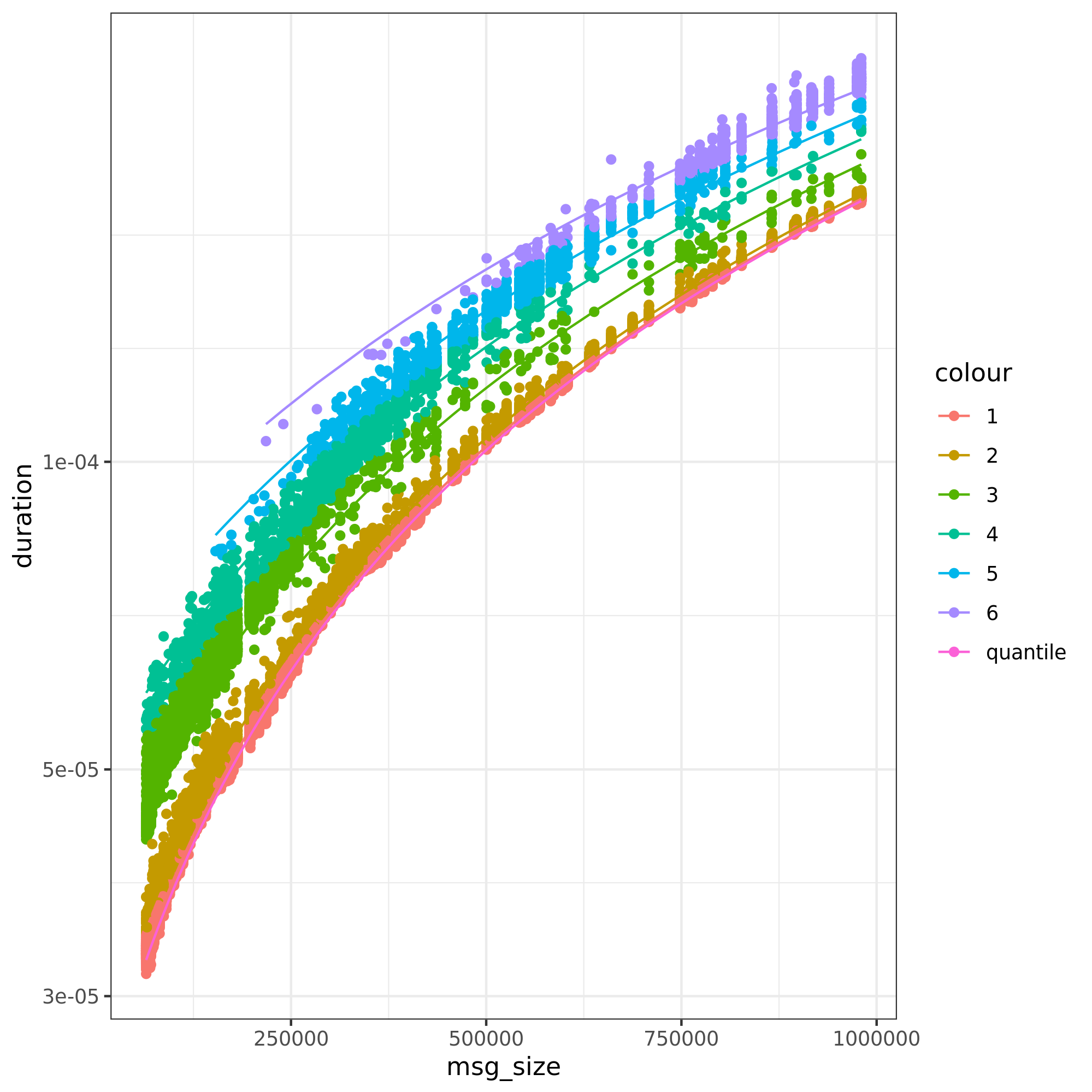
The figure above presents the output for ping-pong. The process involves 4 phases:
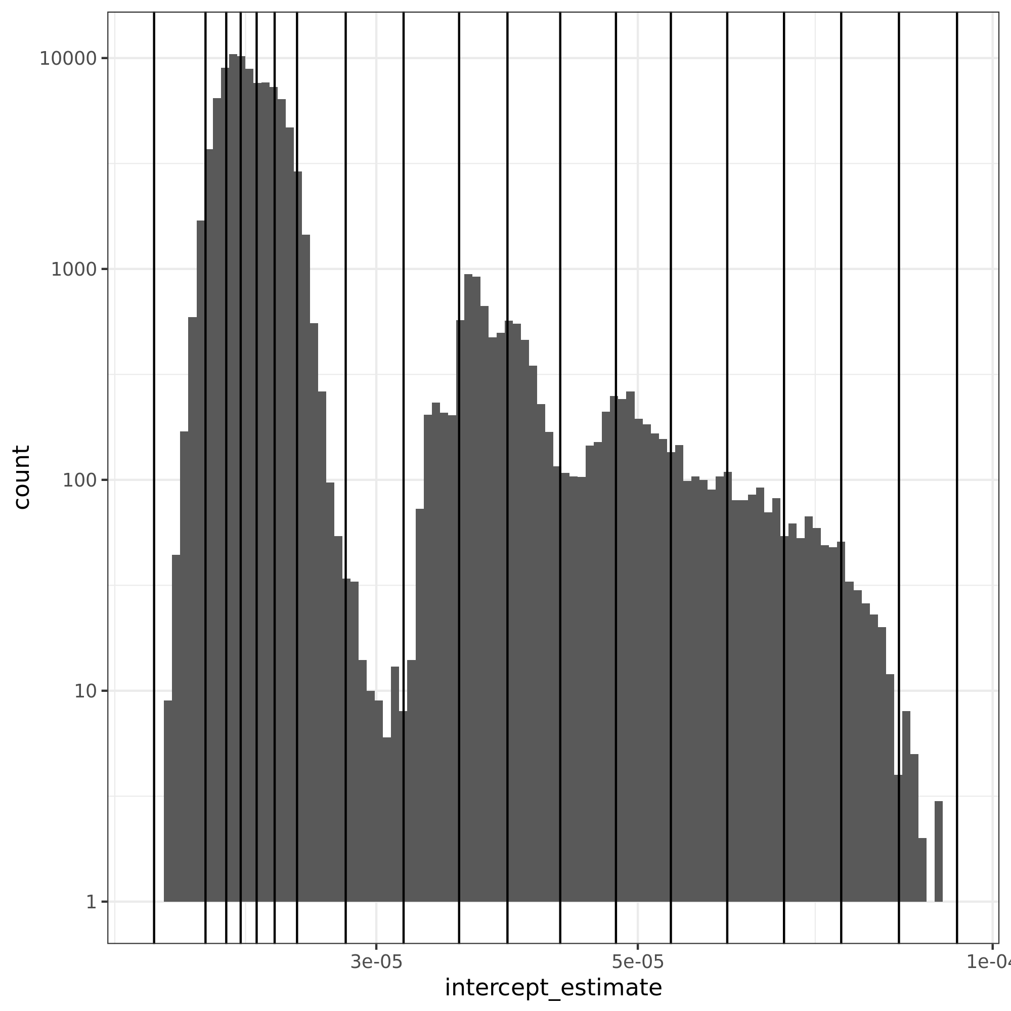
Quantile regression: a quantile regression is made to have our baseline linear model. A quantile regression is used to avoid having negative intercepts and consequently negative estimate duration times.
Intercept residuals: from the quantile regression, we calculate the intercept for each message size (\(intercept = duration - coefficient*msg\_size\))
Ckmeans: creates a set of groups based on our intercept residuals. In the figure, each color represents a group.
Normal distributions: for each group found by ckmeans, we calculate the mean and standard deviation of that group. The probabilities are drawn from the density of each group (points in group/total number of points).
Ping-pong
Ping-pong measures give us the round-trip estimated time, but we need the elapsed time in 1 direction to inject in SimGrid.
For simplicity, we just scale down the normal distributions. However, a proper calculation may be necessary at this step.
pingpong_models["coefficient"] = pingpong_models["coefficient"]/2
pingpong_models["mean"] = pingpong_models["mean"]/2
pingpong_models["sd"] = pingpong_models["sd"]/numpy.sqrt(2)
pingpong_models
| mean | sd | prob | coefficient | min_x | max_x | |
|---|---|---|---|---|---|---|
| 0 | 0.000012 | 4.356809e-07 | 0.499706 | 8.049632e-11 | 63305.0 | 3.402823e+38 |
| 1 | 0.000013 | 5.219426e-07 | 0.385196 | 8.049632e-11 | 63305.0 | 3.402823e+38 |
| 2 | 0.000019 | 1.673437e-06 | 0.073314 | 8.049632e-11 | 63305.0 | 3.402823e+38 |
| 3 | 0.000025 | 2.023256e-06 | 0.024108 | 8.049632e-11 | 63305.0 | 3.402823e+38 |
| 4 | 0.000030 | 2.530620e-06 | 0.011696 | 8.049632e-11 | 63305.0 | 3.402823e+38 |
| 5 | 0.000037 | 3.533823e-06 | 0.005980 | 8.049632e-11 | 63305.0 | 3.402823e+38 |
This table presents the clustering results for Ping-pong. Each line represents a normal distribution that characterizes the noise along with its probability.
At our simulator, we’ll draw our noise following these probabilities/distributions.
Finally, we dump the results in a JSON format. Below, we present the pingpong_ckmeans.json file.
This file will be read by your simulator later to generate the proper factor for network operations.
{'bandwidth_base': 12330818795.43382,
 'latency_base': 1.2924904864614219e-05,
 'seg': [{'mean': 1.1503128856516448e-05,
   'sd': 4.3568091437319533e-07,
   'prob': 0.49970588235294106,
   'coefficient': 8.04963230919345e-11,
   'min_x': 63305.0,
   'max_x': 3.4028234663852886e+38},
  {'mean': 1.2504551284320949e-05,
   'sd': 5.219425841751762e-07,
   'prob': 0.385196078431373,
   'coefficient': 8.04963230919345e-11,
   'min_x': 63305.0,
   'max_x': 3.4028234663852886e+38},
  {'mean': 1.879472592512515e-05,
   'sd': 1.6734369316865939e-06,
   'prob': 0.0733137254901961,
   'coefficient': 8.04963230919345e-11,
   'min_x': 63305.0,
   'max_x': 3.4028234663852886e+38},
  {'mean': 2.451754075327485e-05,
   'sd': 2.0232563328989863e-06,
   'prob': 0.0241078431372549,
   'coefficient': 8.04963230919345e-11,
   'min_x': 63305.0,
   'max_x': 3.4028234663852886e+38},
  {'mean': 3.004149952883e-05,
   'sd': 2.5306204869242285e-06,
   'prob': 0.0116960784313725,
   'coefficient': 8.04963230919345e-11,
   'min_x': 63305.0,
   'max_x': 3.4028234663852886e+38},
  {'mean': 3.688584189653765e-05,
   'sd': 3.5338234385210185e-06,
   'prob': 0.00598039215686275,
   'coefficient': 8.04963230919345e-11,
   'min_x': 63305.0,
   'max_x': 3.4028234663852886e+38}]}
The same is done for each one of the MPI operations, creating the different input files: pingpong_ckmeans.json, isend_ckmeans.json, recv_ckmeans.json, send_ckmeans.json.
4.2. Dhist (alternative 2)
Alternatively, we can model the noise using non-uniform histograms.
Diagonally cut histograms are used in this case, one histogram for each segment.
The noise is later sampled according to these histograms.
Note: For better results, we had to apply a log function on the elapsed time before running the dhist algorithm. However, it’s not clear why this manipulation gives better results.
The figure presents the histogram for the ping-pong operation.
In the x-axis, we have the intercept residuals calculated using the linear models found by pycewise.
The vertical lines are the bins found by dhist. Note that the size of each bin varies depending on their density.
Ping-pong
Ping-pong measures give us the round-trip estimated time, but we need the elapsed time in 1 direction to inject in SimGrid. As we applied the log function on our data, we need a minor trick to calculate the elapsed time.
\(\frac{e^x}{2}\) = \(e^{x + log(\frac{1}{2})}\)
for i in pingpong_dhist:
    i["xbr"] = [v + numpy.log(1/2) for v in i["xbr"]]
    i["coeff"] /= 2

pingpong_dhist = {"bandwidth_base": bandwidth_base, "latency_base" : latency_base, "seg": pingpong_dhist}
pingpong_dhist
{'bandwidth_base': 12330818795.43382,
 'latency_base': 1.2924904864614219e-05,
 'seg': [{'log': True,
   'min_x': 63305.0,
   'max_x': 3.4028234663852886e+38,
   'xbr': [-11.541562041539144,
    -11.441125408005446,
    -11.400596947874545,
    -11.372392420653046,
    -11.341231770713947,
    -11.306064060041345,
    -11.262313043898645,
    -11.167260850740746,
    -11.054191810141747,
    -10.945733341460246,
    -10.851269918507747,
    -10.748196672490847,
    -10.639355545006445,
    -10.532059052445776,
    -10.421953284283596,
    -10.311044865949563,
    -10.199305798019065,
    -10.086544751090685,
    -9.973069718835006],
   'height': [28047.5350565562,
    386265.096035713,
    648676.945998964,
    566809.701663792,
    477810.03815685294,
    342030.173378546,
    41775.283991878,
    972.856932519077,
    10123.6907854913,
    43371.2845877054,
    21848.5405963759,
    9334.7066819517,
    12553.998437911001,
    6766.22135638404,
    5166.42477286285,
    3535.0214326622204,
    1560.8226847324402,
    202.687759084986],
   'coeff': 8.10976153806028e-11}]}
This JSON file is read by the simulator to create the platform and generate the appropriate noise. The same is done for each one of the MPI operations, creating the different input files: pingpong_dhist.json, isend_dhist.json, recv_dhist.json, send_dhist.json.
5. Description of the platform in SimGrid
At this point we have done the analysis and extracted the models in the several JSON files. It’s possible now to create our platform file that will be used by SimGrid later.
The platform is created using the C++ interface from SimGrid. The result is a library file (.so) which is loaded by SimGrid when running the application.
The best to understand is reading the C++ code in docs/source/tuto_network_calibration, the main files are:
dahu_platform_ckmeans.cpp: create the dahu platform using the JSON files from ckmeans.
dahu_platform_dhist.cpp: same for dhist output.
Utils.cpp/Utils.hpp: some auxiliary classes used by both platforms to handle the segmentation and sampling.
CMakeLists.txt: create the shared library to be loaded by SimGrid
Feel free to re-use and adapt these files according to your needs.
6. SimGrid execution and comparison
6.1. Execution
Ckmeans.1d.dp and Dhist
The execution is similar for both modes. The only change is the platform library to be used: libdahu_ckmeans.so or libdhist.so.
%%bash

cd /source/simgrid.git/docs/source/tuto_network_calibration/

smpirun --cfg=smpi/simulate-computation:0 \
    --cfg=smpi/display-timing:yes \
    -platform ./libdahu_ckmeans.so \
    -hostfile /tmp/host.txt -np 2 \
    /source/platform-calibration/src/calibration/calibrate -d /tmp/exp -m 1 -M 1000000 -p exp -s /tmp/exp.csv
Read bandwidth_base: 1.233082e+10 latency_base: 1.292490e-05
Starting parsing file: pingpong_ckmeans.json
Starting parsing file: send_ckmeans.json
Starting parsing file: isend_ckmeans.json
Starting parsing file: recv_ckmeans.json
[0] MPI initialized
[0] nb_exp=115200, largest_size=980284
[0] Alloc size: 1960568
[1] MPI initialized
[1] nb_exp=115200, largest_size=980284
[1] Alloc size: 1960568
[0.000000] [xbt_cfg/INFO] Configuration change: Set 'smpi/privatization' to '1'
[0.000000] [xbt_cfg/INFO] Configuration change: Set 'smpi/np' to '2'
[0.000000] [xbt_cfg/INFO] Configuration change: Set 'smpi/hostfile' to '/tmp/host.txt'
[0.000000] [xbt_cfg/INFO] Configuration change: Set 'precision/work-amount' to '1e-9'
[0.000000] [xbt_cfg/INFO] Configuration change: Set 'network/model' to 'SMPI'
[0.000000] [xbt_cfg/INFO] Configuration change: Set 'smpi/simulate-computation' to '0'
[0.000000] [xbt_cfg/INFO] Configuration change: Set 'smpi/display-timing' to 'yes'
[0.000000] [xbt_cfg/INFO] Configuration change: Set 'smpi/tmpdir' to '/tmp'
[0.000000] [smpi_config/INFO] You did not set the power of the host running the simulation.  The timings will certainly not be accurate.  Use the option "--cfg=smpi/host-speed:<flops>" to set its value.  Check https://simgrid.org/doc/latest/Configuring_SimGrid.html#automatic-benchmarking-of-smpi-code for more information.
[6.845963] [smpi_utils/INFO] Simulated time: 6.84596 seconds.

The simulation took 71.6111 seconds (after parsing and platform setup)
1.77771 seconds were actual computation of the application
6.2. Comparison
Finally, let’s compare the SimGrid results the real ones. The red points are the real data while the blue ones are the output from our simulator.
Ckmeans.1d.dp
Dhist
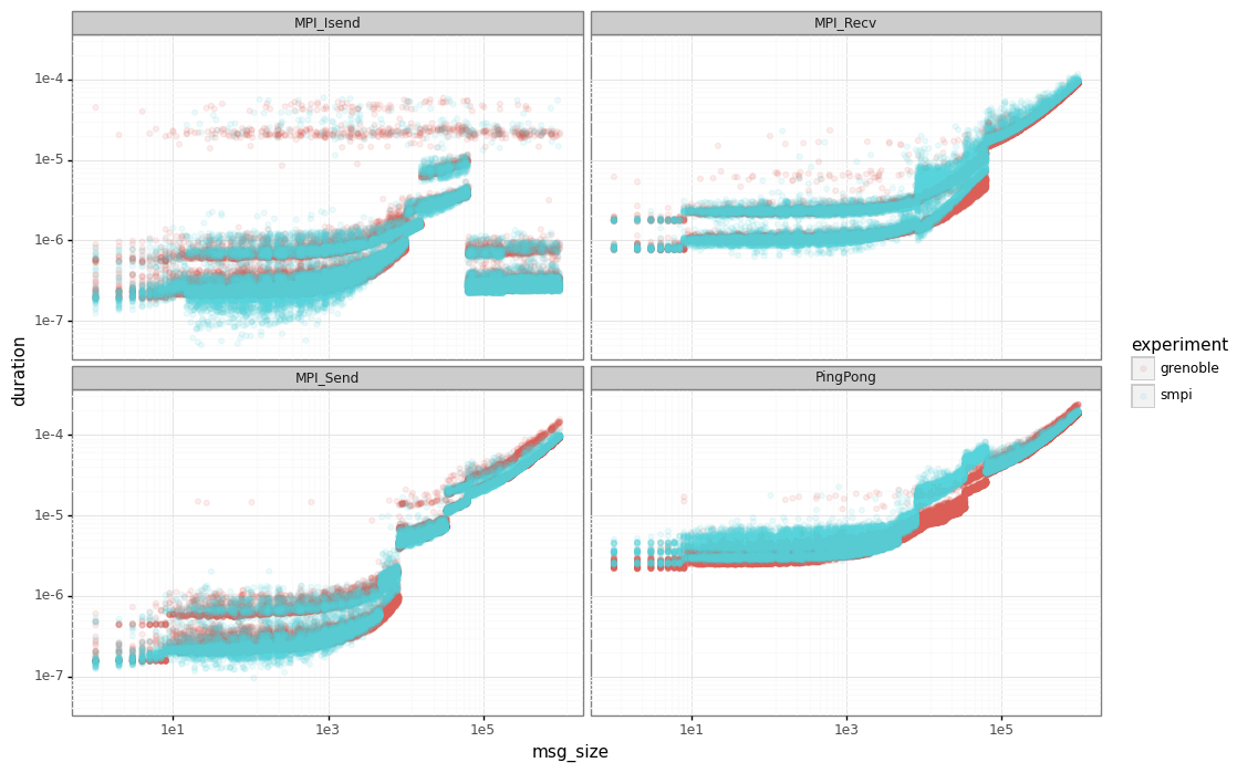
Ping-Pong
Note that for ping-ping tests, we have an important gap between the real performance (in red) and SimGrid (in blue) for messages below our sync/async threshold (63305).
This behavior is explained by how we measure the extra cost for each MPI_Send/MPI_Recv operations.
In calibrate.c in platform-calibration, the ping-pong test is as follows (considering the processes are synchronized):
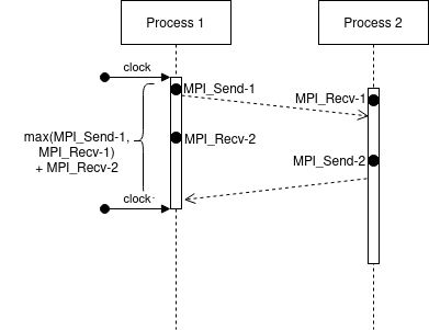
We can see that we measure the delay at Process 1, just before the first MPI_Send-1 until the end of respective MPI_Recv-2. Moreover, the extra cost of MPI operations is paid concurrently with the network communication cost.
In this case, it doesn’t matter when the MPI_Send-2 will finish. Despite we expect that it finished before the MPI_Recv-2, we couldn’t be sure.
Also, both processes are running in parallel, so we can expect that the measure time will be: \(max(\text{MPI_Send-1}, \text{MPI_Recv-1}) + \text{MPI_Recv-2}\) - \(max(\text{MPI_Send-1}, \text{MPI_Recv-1})\): since we cannot start MPI_Recv-2 or MPI_Send_2 before finishing both commands - \(\text{MPI_Recv-2}\): because we measure just after the finishing of this receive
However, the simulation world is a little more stable. The same communication occurs in the following way:
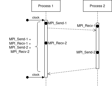
In SimGrid, the extra costs are paid sequentially. That means, initially we pay the extra cost for MPI_Send-1, after the network communication cost, followed by the extra cost for MPI-Recv-1.
This effect leads to a total time of: MPI_Send-1 + MPI_Recv-1 + MPI_Send-2 + MPI_Recv-2 which is slightly higher than the real cost.
The same doesn’t happen for largest messages because we don’t pay the extra overhead cost for each MPI operation (the communication is limited by the network capacity).
I/O calibration
Introduction
This tutorial presents how to perform faithful IO experiments in SimGrid. It is based on the paper “Adding Storage Simulation Capacities to the SimGridToolkit: Concepts, Models, and API”.
The paper presents a series of experiments to analyze the performance of IO operations (read/write) on different kinds of disks (SATA, SAS, SSD). In this tutorial, we present a detailed example of how to extract experimental data to simulate: i) performance degradation with concurrent operations (Fig. 8 in the paper) and ii) variability in IO operations (Fig. 5 to 7).
Link for paper: https://hal.inria.fr/hal-01197128
Link for data: https://figshare.com/articles/dataset/Companion_of_the_SimGrid_storage_modeling_article/1175156
Disclaimer:
The purpose of this document is to illustrate how we can extract data from experiments and inject on SimGrid. However, the data shown on this page may not reflect the reality.
You must run similar experiments on your hardware to get realistic data for your context.
SimGrid has been in active development since the paper release in 2015, thus the XML description used in the paper may have evolved while MSG was superseeded by S4U since then.
Running this tutorial
A Dockerfile is available in docs/source/tuto_disk. It allows you to
re-run this tutorial. For that, build the image and run the container:
docker build -t tuto_disk .docker run -it tuto_disk
Analyzing the experimental data
We start by analyzing and extracting the real data available.
Scripts
We use a special method to create non-uniform histograms to represent the noise in IO operations.
Unable to install the library properly, I copied the important methods here.
Copied from: https://rdrr.io/github/dlebauer/pecan-priors/src/R/plots.R
Data preparation
Some initial configurations/list of packages.
library(jsonlite)
library(ggplot2)
library(plyr)
library(dplyr)
library(gridExtra)

IO_INFO = list()
Use suppressPackageStartupMessages() to eliminate package startup
messages.

Attaching package: 'dplyr'

The following objects are masked from 'package:plyr':

    arrange, count, desc, failwith, id, mutate, rename, summarise,
    summarize

The following objects are masked from 'package:stats':

    filter, lag

The following objects are masked from 'package:base':

    intersect, setdiff, setequal, union

Attaching package: 'gridExtra'

The following object is masked from 'package:dplyr':

    combine
This was copied from the sg_storage_ccgrid15.org available at the
figshare of the paper. Before executing this code, please download and
decompress the appropriate file.
curl -O -J -L "https://ndownloader.figshare.com/files/1928095"
tar xfz bench.tgz
Preparing data for varialiby analysis.
clean_up <- function (df, infra){
names(df) <- c("Hostname","Date","DirectIO","IOengine","IOscheduler","Error","Operation","Jobs","BufferSize","FileSize","Runtime","Bandwidth","BandwidthMin","BandwidthMax","Latency", "LatencyMin", "LatencyMax","IOPS")
df=subset(df,Error=="0")
df=subset(df,DirectIO=="1")
df <- merge(df,infra,by="Hostname")
df$Hostname = sapply(strsplit(df$Hostname, "[.]"), "[", 1)
df$HostModel = paste(df$Hostname, df$Model, sep=" - ")
df$Duration = df$Runtime/1000 # fio outputs runtime in msec, we want to display seconds
df$Size = df$FileSize/1024/1024
df=subset(df,Duration!=0.000)
df$Bwi=df$Duration/df$Size
df[df$Operation=="read",]$Operation<- "Read"
df[df$Operation=="write",]$Operation<- "Write"
return(df)
}

grenoble <- read.csv('./bench/grenoble.csv', header=FALSE,sep = ";",
stringsAsFactors=FALSE)
luxembourg <- read.csv('./bench/luxembourg.csv', header=FALSE,sep = ";",  stringsAsFactors=FALSE)
nancy <- read.csv('./bench/nancy.csv', header=FALSE,sep = ";",  stringsAsFactors=FALSE)
all <- rbind(grenoble,nancy, luxembourg)
infra <- read.csv('./bench/infra.csv', header=FALSE,sep = ";",  stringsAsFactors=FALSE)
names(infra) <- c("Hostname","Model","DiskSize")

all = clean_up(all, infra)
griffon = subset(all,grepl("^griffon", Hostname))
griffon$Cluster <-"Griffon (SATA II)"
edel = subset(all,grepl("^edel", Hostname))
edel$Cluster<-"Edel (SSD)"

df = rbind(griffon[griffon$Jobs=="1" & griffon$IOscheduler=="cfq",],
           edel[edel$Jobs=="1" & edel$IOscheduler=="cfq",])
#Get rid off of 64 Gb disks of Edel as they behave differently (used to be "edel-51")
df = df[!(grepl("^Edel",df$Cluster) & df$DiskSize=="64 GB"),]
Preparing data for concurrent analysis.
dfc = rbind(griffon[griffon$Jobs>1 & griffon$IOscheduler=="cfq",],
           edel[edel$Jobs>1 & edel$IOscheduler=="cfq",])
dfc2 = rbind(griffon[griffon$Jobs==1 & griffon$IOscheduler=="cfq",],
           edel[edel$Jobs==1 & edel$IOscheduler=="cfq",])
dfc = rbind(dfc,dfc2[sample(nrow(dfc2),size=200),])

dd <- data.frame(
      Hostname="??",
      Date = NA, #tmpl$Date,
      DirectIO = NA,
      IOengine = NA,
      IOscheduler = NA,
      Error = 0,
      Operation = NA, #tmpl$Operation,
      Jobs = NA, # #d$nb.of.concurrent.access,
      BufferSize = NA, #d$bs,
      FileSize = NA, #d$size,
      Runtime = NA,
      Bandwidth = NA,
      BandwidthMin = NA,
      BandwidthMax = NA,
      Latency = NA,
      LatencyMin = NA,
      LatencyMax = NA,
      IOPS = NA,
      Model = NA, #tmpl$Model,
      DiskSize = NA, #tmpl$DiskSize,
      HostModel = NA,
      Duration = NA, #d$time,
      Size = NA,
      Bwi = NA,
      Cluster = NA) #tmpl$Cluster)

dd$Size = dd$FileSize/1024/1024
dd$Bwi = dd$Duration/dd$Size

dfc = rbind(dfc, dd)
# Let's get rid of small files!
dfc = subset(dfc,Size >= 10)
# Let's get rid of 64Gb edel disks
dfc = dfc[!(grepl("^Edel",dfc$Cluster) & dfc$DiskSize=="64 GB"),]

dfc$TotalSize=dfc$Size * dfc$Jobs
dfc$BW = (dfc$TotalSize) / dfc$Duration
dfc = dfc[dfc$BW>=20,] # get rid of one point that is typically an outlier and does not make sense

dfc$method="lm"
dfc[dfc$Cluster=="Edel (SSD)"  & dfc$Operation=="Read",]$method="loess"

dfc[dfc$Cluster=="Edel (SSD)"  & dfc$Operation=="Write" & dfc$Jobs ==1,]$method="lm"
dfc[dfc$Cluster=="Edel (SSD)"  & dfc$Operation=="Write" & dfc$Jobs ==1,]$method=""

dfc[dfc$Cluster=="Griffon (SATA II)" & dfc$Operation=="Write",]$method="lm"
dfc[dfc$Cluster=="Griffon (SATA II)"  & dfc$Operation=="Write" & dfc$Jobs ==1,]$method=""

dfd = dfc[dfc$Operation=="Write" & dfc$Jobs ==1 &
          (dfc$Cluster %in% c("Griffon (SATA II)", "Edel (SSD)")),]
dfd = ddply(dfd,c("Cluster","Operation","Jobs","DiskSize"), summarize,
            mean = mean(BW), num = length(BW), sd = sd(BW))
dfd$BW=dfd$mean
dfd$ci = 2*dfd$sd/sqrt(dfd$num)

dfrange=ddply(dfc,c("Cluster","Operation","DiskSize"), summarize,
            max = max(BW))
dfrange=ddply(dfrange,c("Cluster","DiskSize"), mutate,
            BW = max(max))
dfrange$Jobs=16
Griffon (SATA)
Modeling resource sharing w/ concurrent access
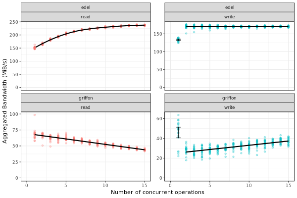
This figure presents the overall performance of IO operation with concurrent access to the disk. Note that the image is different from the one in the paper. Probably, we need to further clean the available data to obtain exaclty the same results.
ggplot(data=dfc,aes(x=Jobs,y=BW, color=Operation)) + theme_bw() +
  geom_point(alpha=.3) +
  geom_point(data=dfrange, size=0) +
  facet_wrap(Cluster~Operation,ncol=2,scale="free_y")+ # ) + #
  geom_smooth(data=dfc[dfc$method=="loess",], color="black", method=loess,se=TRUE,fullrange=T) +
  geom_smooth(data=dfc[dfc$method=="lm",], color="black", method=lm,se=TRUE) +
  geom_point(data=dfd, aes(x=Jobs,y=BW),color="black",shape=21,fill="white") +
  geom_errorbar(data=dfd, aes(x=Jobs, ymin=BW-ci, ymax=BW+ci),color="black",width=.6) +
  xlab("Number of concurrent operations") + ylab("Aggregated Bandwidth (MiB/s)")  + guides(color=FALSE)  + xlim(0,NA) + ylim(0,NA)
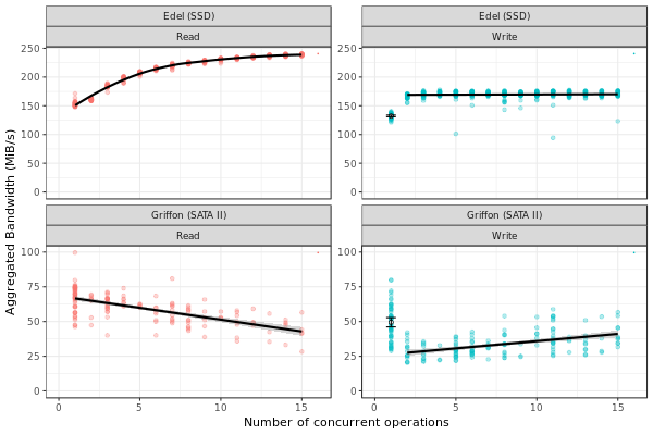
Read
Getting read data for Griffon from 1 to 15 concurrent reads.
deg_griffon = dfc %>% filter(grepl("^Griffon", Cluster)) %>% filter(Operation == "Read")
model = lm(BW~Jobs, data = deg_griffon)
IO_INFO[["griffon"]][["degradation"]][["read"]] = predict(model,data.frame(Jobs=seq(1,15)))

toJSON(IO_INFO, pretty = TRUE)
{
  "griffon": {
    "degradation": {
      "read": [66.6308, 64.9327, 63.2346, 61.5365, 59.8384, 58.1403, 56.4423, 54.7442, 53.0461, 51.348, 49.6499, 47.9518, 46.2537, 44.5556, 42.8575]
    }
  }
}
Write
Same for write operations.
deg_griffon = dfc %>% filter(grepl("^Griffon", Cluster)) %>% filter(Operation == "Write") %>% filter(Jobs > 2)
mean_job_1 = dfc %>% filter(grepl("^Griffon", Cluster)) %>% filter(Operation == "Write") %>% filter(Jobs == 1) %>% summarize(mean = mean(BW))
model = lm(BW~Jobs, data = deg_griffon)
IO_INFO[["griffon"]][["degradation"]][["write"]] = c(mean_job_1$mean, predict(model,data.frame(Jobs=seq(2,15))))
toJSON(IO_INFO, pretty = TRUE)
{
  "griffon": {
    "degradation": {
      "read": [66.6308, 64.9327, 63.2346, 61.5365, 59.8384, 58.1403, 56.4423, 54.7442, 53.0461, 51.348, 49.6499, 47.9518, 46.2537, 44.5556, 42.8575],
      "write": [49.4576, 26.5981, 27.7486, 28.8991, 30.0495, 31.2, 32.3505, 33.501, 34.6515, 35.8019, 36.9524, 38.1029, 39.2534, 40.4038, 41.5543]
    }
  }
}
Modeling read/write bandwidth variability
Fig.5 in the paper presents the noise in the read/write operations in the Griffon SATA disk.
The paper uses regular histogram to illustrate the distribution of the effective bandwidth. However, in this tutorial, we use dhist (https://rdrr.io/github/dlebauer/pecan-priors/man/dhist.html) to have a more precise information over the highly dense areas around the mean.
Read
First, we present the histogram for read operations.
griffon_read = df %>% filter(grepl("^Griffon", Cluster)) %>% filter(Operation == "Read") %>% select(Bwi)
dhist(1/griffon_read$Bwi)
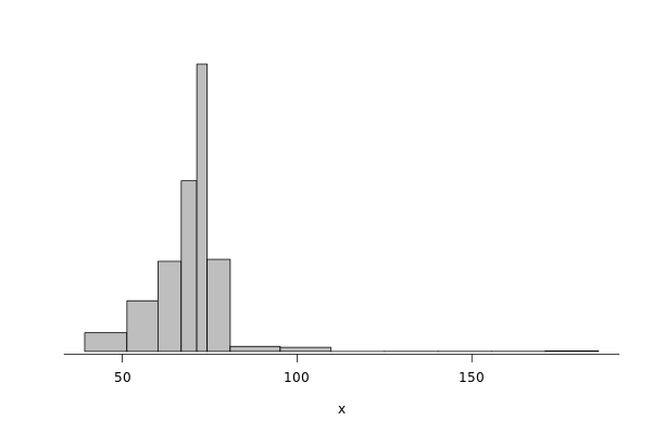
Saving it to be exported in json format.
griffon_read_dhist = dhist(1/griffon_read$Bwi, plot=FALSE)
IO_INFO[["griffon"]][["noise"]][["read"]] = c(breaks=list(griffon_read_dhist$xbr), heights=list(unclass(griffon_read_dhist$heights)))
IO_INFO[["griffon"]][["read_bw"]] = mean(1/griffon_read$Bwi)
toJSON(IO_INFO, pretty = TRUE)
Warning message:
In hist.default(x, breaks = cut.pt, plot = FALSE, probability = TRUE) :
  argument 'probability' is not made use of

{
  "griffon": {
    "degradation": {
      "read": [66.6308, 64.9327, 63.2346, 61.5365, 59.8384, 58.1403, 56.4423, 54.7442, 53.0461, 51.348, 49.6499, 47.9518, 46.2537, 44.5556, 42.8575],
      "write": [49.4576, 26.5981, 27.7486, 28.8991, 30.0495, 31.2, 32.3505, 33.501, 34.6515, 35.8019, 36.9524, 38.1029, 39.2534, 40.4038, 41.5543]
    },
    "noise": {
      "read": {
    "breaks": [39.257, 51.3413, 60.2069, 66.8815, 71.315, 74.2973, 80.8883, 95.1944, 109.6767, 125.0231, 140.3519, 155.6807, 171.0094, 186.25],
    "heights": [15.3091, 41.4578, 73.6826, 139.5982, 235.125, 75.3357, 4.1241, 3.3834, 0, 0.0652, 0.0652, 0.0652, 0.3937]
      }
    },
    "read_bw": [68.5425]
  }
}
Write
Same analysis for write operations.
griffon_write = df %>% filter(grepl("^Griffon", Cluster)) %>% filter(Operation == "Write") %>% select(Bwi)
dhist(1/griffon_write$Bwi)
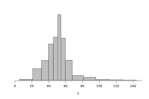
griffon_write_dhist = dhist(1/griffon_write$Bwi, plot=FALSE)
IO_INFO[["griffon"]][["noise"]][["write"]] = c(breaks=list(griffon_write_dhist$xbr), heights=list(unclass(griffon_write_dhist$heights)))
IO_INFO[["griffon"]][["write_bw"]] = mean(1/griffon_write$Bwi)
toJSON(IO_INFO, pretty = TRUE)
Warning message:
In hist.default(x, breaks = cut.pt, plot = FALSE, probability = TRUE) :
  argument 'probability' is not made use of

{
  "griffon": {
    "degradation": {
      "read": [66.6308, 64.9327, 63.2346, 61.5365, 59.8384, 58.1403, 56.4423, 54.7442, 53.0461, 51.348, 49.6499, 47.9518, 46.2537, 44.5556, 42.8575],
      "write": [49.4576, 26.5981, 27.7486, 28.8991, 30.0495, 31.2, 32.3505, 33.501, 34.6515, 35.8019, 36.9524, 38.1029, 39.2534, 40.4038, 41.5543]
    },
    "noise": {
      "read": {
    "breaks": [39.257, 51.3413, 60.2069, 66.8815, 71.315, 74.2973, 80.8883, 95.1944, 109.6767, 125.0231, 140.3519, 155.6807, 171.0094, 186.25],
    "heights": [15.3091, 41.4578, 73.6826, 139.5982, 235.125, 75.3357, 4.1241, 3.3834, 0, 0.0652, 0.0652, 0.0652, 0.3937]
      },
      "write": {
    "breaks": [5.2604, 21.0831, 31.4773, 39.7107, 45.5157, 50.6755, 54.4726, 59.7212, 67.8983, 81.2193, 95.6333, 111.5864, 127.8409, 144.3015],
    "heights": [1.7064, 22.6168, 38.613, 70.8008, 84.4486, 128.5118, 82.3692, 39.1431, 9.2256, 5.6195, 1.379, 0.6429, 0.1549]
      }
    },
    "read_bw": [68.5425],
    "write_bw": [50.6045]
  }
}
Edel (SSD)
This section presents the exactly same analysis for the Edel SSDs.
Modeling resource sharing w/ concurrent access
Read
Getting read data for Edel from 1 to 15 concurrent operations.
deg_edel = dfc %>% filter(grepl("^Edel", Cluster)) %>% filter(Operation == "Read")
model = loess(BW~Jobs, data = deg_edel)
IO_INFO[["edel"]][["degradation"]][["read"]] = predict(model,data.frame(Jobs=seq(1,15)))
toJSON(IO_INFO, pretty = TRUE)
{
  "griffon": {
    "degradation": {
      "read": [66.6308, 64.9327, 63.2346, 61.5365, 59.8384, 58.1403, 56.4423, 54.7442, 53.0461, 51.348, 49.6499, 47.9518, 46.2537, 44.5556, 42.8575],
      "write": [49.4576, 26.5981, 27.7486, 28.8991, 30.0495, 31.2, 32.3505, 33.501, 34.6515, 35.8019, 36.9524, 38.1029, 39.2534, 40.4038, 41.5543]
    },
    "noise": {
      "read": {
    "breaks": [39.257, 51.3413, 60.2069, 66.8815, 71.315, 74.2973, 80.8883, 95.1944, 109.6767, 125.0231, 140.3519, 155.6807, 171.0094, 186.25],
    "heights": [15.3091, 41.4578, 73.6826, 139.5982, 235.125, 75.3357, 4.1241, 3.3834, 0, 0.0652, 0.0652, 0.0652, 0.3937]
      },
      "write": {
    "breaks": [5.2604, 21.0831, 31.4773, 39.7107, 45.5157, 50.6755, 54.4726, 59.7212, 67.8983, 81.2193, 95.6333, 111.5864, 127.8409, 144.3015],
    "heights": [1.7064, 22.6168, 38.613, 70.8008, 84.4486, 128.5118, 82.3692, 39.1431, 9.2256, 5.6195, 1.379, 0.6429, 0.1549]
      }
    },
    "read_bw": [68.5425],
    "write_bw": [50.6045]
  },
  "edel": {
    "degradation": {
      "read": [150.5119, 167.4377, 182.2945, 195.1004, 205.8671, 214.1301, 220.411, 224.6343, 227.7141, 230.6843, 233.0923, 235.2027, 236.8369, 238.0249, 238.7515]
    }
  }
}
Write
Same for write operations.
deg_edel = dfc %>% filter(grepl("^Edel", Cluster)) %>% filter(Operation == "Write") %>% filter(Jobs > 2)
mean_job_1 = dfc %>% filter(grepl("^Edel", Cluster)) %>% filter(Operation == "Write") %>% filter(Jobs == 1) %>% summarize(mean = mean(BW))
model = lm(BW~Jobs, data = deg_edel)
IO_INFO[["edel"]][["degradation"]][["write"]] = c(mean_job_1$mean, predict(model,data.frame(Jobs=seq(2,15))))
toJSON(IO_INFO, pretty = TRUE)
{
  "griffon": {
    "degradation": {
      "read": [66.6308, 64.9327, 63.2346, 61.5365, 59.8384, 58.1403, 56.4423, 54.7442, 53.0461, 51.348, 49.6499, 47.9518, 46.2537, 44.5556, 42.8575],
      "write": [49.4576, 26.5981, 27.7486, 28.8991, 30.0495, 31.2, 32.3505, 33.501, 34.6515, 35.8019, 36.9524, 38.1029, 39.2534, 40.4038, 41.5543]
    },
    "noise": {
      "read": {
    "breaks": [39.257, 51.3413, 60.2069, 66.8815, 71.315, 74.2973, 80.8883, 95.1944, 109.6767, 125.0231, 140.3519, 155.6807, 171.0094, 186.25],
    "heights": [15.3091, 41.4578, 73.6826, 139.5982, 235.125, 75.3357, 4.1241, 3.3834, 0, 0.0652, 0.0652, 0.0652, 0.3937]
      },
      "write": {
    "breaks": [5.2604, 21.0831, 31.4773, 39.7107, 45.5157, 50.6755, 54.4726, 59.7212, 67.8983, 81.2193, 95.6333, 111.5864, 127.8409, 144.3015],
    "heights": [1.7064, 22.6168, 38.613, 70.8008, 84.4486, 128.5118, 82.3692, 39.1431, 9.2256, 5.6195, 1.379, 0.6429, 0.1549]
      }
    },
    "read_bw": [68.5425],
    "write_bw": [50.6045]
  },
  "edel": {
    "degradation": {
      "read": [150.5119, 167.4377, 182.2945, 195.1004, 205.8671, 214.1301, 220.411, 224.6343, 227.7141, 230.6843, 233.0923, 235.2027, 236.8369, 238.0249, 238.7515],
      "write": [132.2771, 170.174, 170.137, 170.1, 170.063, 170.026, 169.9889, 169.9519, 169.9149, 169.8779, 169.8408, 169.8038, 169.7668, 169.7298, 169.6927]
    }
  }
}
Modeling read/write bandwidth variability
Read
edel_read = df %>% filter(grepl("^Edel", Cluster)) %>% filter(Operation == "Read") %>% select(Bwi)
dhist(1/edel_read$Bwi)
Saving it to be exported in json format.
edel_read_dhist = dhist(1/edel_read$Bwi, plot=FALSE)
IO_INFO[["edel"]][["noise"]][["read"]] = c(breaks=list(edel_read_dhist$xbr), heights=list(unclass(edel_read_dhist$heights)))
IO_INFO[["edel"]][["read_bw"]] = mean(1/edel_read$Bwi)
toJSON(IO_INFO, pretty = TRUE)
Warning message:
In hist.default(x, breaks = cut.pt, plot = FALSE, probability = TRUE) :
  argument 'probability' is not made use of

{
  "griffon": {
    "degradation": {
      "read": [66.6308, 64.9327, 63.2346, 61.5365, 59.8384, 58.1403, 56.4423, 54.7442, 53.0461, 51.348, 49.6499, 47.9518, 46.2537, 44.5556, 42.8575],
      "write": [49.4576, 26.5981, 27.7486, 28.8991, 30.0495, 31.2, 32.3505, 33.501, 34.6515, 35.8019, 36.9524, 38.1029, 39.2534, 40.4038, 41.5543]
    },
    "noise": {
      "read": {
    "breaks": [39.257, 51.3413, 60.2069, 66.8815, 71.315, 74.2973, 80.8883, 95.1944, 109.6767, 125.0231, 140.3519, 155.6807, 171.0094, 186.25],
    "heights": [15.3091, 41.4578, 73.6826, 139.5982, 235.125, 75.3357, 4.1241, 3.3834, 0, 0.0652, 0.0652, 0.0652, 0.3937]
      },
      "write": {
    "breaks": [5.2604, 21.0831, 31.4773, 39.7107, 45.5157, 50.6755, 54.4726, 59.7212, 67.8983, 81.2193, 95.6333, 111.5864, 127.8409, 144.3015],
    "heights": [1.7064, 22.6168, 38.613, 70.8008, 84.4486, 128.5118, 82.3692, 39.1431, 9.2256, 5.6195, 1.379, 0.6429, 0.1549]
      }
    },
    "read_bw": [68.5425],
    "write_bw": [50.6045]
  },
  "edel": {
    "degradation": {
      "read": [150.5119, 167.4377, 182.2945, 195.1004, 205.8671, 214.1301, 220.411, 224.6343, 227.7141, 230.6843, 233.0923, 235.2027, 236.8369, 238.0249, 238.7515],
      "write": [132.2771, 170.174, 170.137, 170.1, 170.063, 170.026, 169.9889, 169.9519, 169.9149, 169.8779, 169.8408, 169.8038, 169.7668, 169.7298, 169.6927]
    },
    "noise": {
      "read": {
    "breaks": [104.1667, 112.3335, 120.5003, 128.6671, 136.8222, 144.8831, 149.6239, 151.2937, 154.0445, 156.3837, 162.3555, 170.3105, 178.3243],
    "heights": [0.1224, 0.1224, 0.1224, 0.2452, 1.2406, 61.6128, 331.2201, 167.6488, 212.1086, 31.3996, 2.3884, 1.747]
      }
    },
    "read_bw": [152.7139]
  }
}
Write
edel_write = df %>% filter(grepl("^Edel", Cluster)) %>% filter(Operation == "Write") %>% select(Bwi)
dhist(1/edel_write$Bwi)
Saving it to be exported later.
edel_write_dhist = dhist(1/edel_write$Bwi, plot=FALSE)
IO_INFO[["edel"]][["noise"]][["write"]] = c(breaks=list(edel_write_dhist$xbr), heights=list(unclass(edel_write_dhist$heights)))
IO_INFO[["edel"]][["write_bw"]] = mean(1/edel_write$Bwi)
toJSON(IO_INFO, pretty = TRUE)
Warning message:
In hist.default(x, breaks = cut.pt, plot = FALSE, probability = TRUE) :
  argument 'probability' is not made use of

{
  "griffon": {
    "degradation": {
      "read": [66.6308, 64.9327, 63.2346, 61.5365, 59.8384, 58.1403, 56.4423, 54.7442, 53.0461, 51.348, 49.6499, 47.9518, 46.2537, 44.5556, 42.8575],
      "write": [49.4576, 26.5981, 27.7486, 28.8991, 30.0495, 31.2, 32.3505, 33.501, 34.6515, 35.8019, 36.9524, 38.1029, 39.2534, 40.4038, 41.5543]
    },
    "noise": {
      "read": {
    "breaks": [39.257, 51.3413, 60.2069, 66.8815, 71.315, 74.2973, 80.8883, 95.1944, 109.6767, 125.0231, 140.3519, 155.6807, 171.0094, 186.25],
    "heights": [15.3091, 41.4578, 73.6826, 139.5982, 235.125, 75.3357, 4.1241, 3.3834, 0, 0.0652, 0.0652, 0.0652, 0.3937]
      },
      "write": {
    "breaks": [5.2604, 21.0831, 31.4773, 39.7107, 45.5157, 50.6755, 54.4726, 59.7212, 67.8983, 81.2193, 95.6333, 111.5864, 127.8409, 144.3015],
    "heights": [1.7064, 22.6168, 38.613, 70.8008, 84.4486, 128.5118, 82.3692, 39.1431, 9.2256, 5.6195, 1.379, 0.6429, 0.1549]
      }
    },
    "read_bw": [68.5425],
    "write_bw": [50.6045]
  },
  "edel": {
    "degradation": {
      "read": [150.5119, 167.4377, 182.2945, 195.1004, 205.8671, 214.1301, 220.411, 224.6343, 227.7141, 230.6843, 233.0923, 235.2027, 236.8369, 238.0249, 238.7515],
      "write": [132.2771, 170.174, 170.137, 170.1, 170.063, 170.026, 169.9889, 169.9519, 169.9149, 169.8779, 169.8408, 169.8038, 169.7668, 169.7298, 169.6927]
    },
    "noise": {
      "read": {
    "breaks": [104.1667, 112.3335, 120.5003, 128.6671, 136.8222, 144.8831, 149.6239, 151.2937, 154.0445, 156.3837, 162.3555, 170.3105, 178.3243],
    "heights": [0.1224, 0.1224, 0.1224, 0.2452, 1.2406, 61.6128, 331.2201, 167.6488, 212.1086, 31.3996, 2.3884, 1.747]
      },
      "write": {
    "breaks": [70.9593, 79.9956, 89.0654, 98.085, 107.088, 115.9405, 123.5061, 127.893, 131.083, 133.6696, 135.7352, 139.5932, 147.4736],
    "heights": [0.2213, 0, 0.3326, 0.4443, 1.4685, 11.8959, 63.869, 110.286, 149.9741, 202.887, 80.8298, 9.0298]
      }
    },
    "read_bw": [152.7139],
    "write_bw": [131.7152]
  }
}
Exporting to JSON
Finally, let’s save it to a file to be opened by our simulator.
json = toJSON(IO_INFO, pretty = TRUE)
cat(json, file="IO_noise.json")
Injecting this data in SimGrid
To mimic this behavior in SimGrid, we use two features in the platform
description: non-linear sharing policy and bandwidth factors. For more
details, please see the source code in tuto_disk.cpp.
Modeling resource sharing w/ concurrent access
The set_sharing_policy method allows the user to set a callback to
dynamically change the disk capacity. The callback is called each time
SimGrid will share the disk between a set of I/O operations.
The callback has access to the number of activities sharing the resource and its current capacity. It must return the new resource’s capacity.
static double disk_dynamic_sharing(double capacity, int n)
{
   return capacity; //useless callback
}

auto* disk = host->add_disk("dump", 1e6, 1e6);
disk->set_sharing_policy(sg4::Disk::Operation::READ, sg4::Disk::SharingPolicy::NONLINEAR, &disk_dynamic_sharing);
Modeling read/write bandwidth variability
The noise in I/O operations can be obtained by applying a factor to the I/O bandwidth of the disk. This factor is applied when we update the remaining amount of bytes to be transferred, increasing or decreasing the effective disk bandwidth.
The set_factor method allows the user to set a callback to
dynamically change the factor to be applied for each I/O operation.
The callback has access to size of the operation and its type (read or
write). It must return a multiply factor (e.g. 1.0 for doing nothing).
static double disk_variability(sg_size_t size, sg4::Io::OpType op)
{
   return 1.0; //useless callback
}

auto* disk = host->add_disk("dump", 1e6, 1e6);
disk->set_factor_cb(&disk_variability);
Running our simulation
The binary was compiled in the provided docker container.
./tuto_disk > ./simgrid_disk.csv
Analyzing the SimGrid results
The figure below presents the results obtained by SimGrid.
The experiment performs I/O operations, varying the number of concurrent operations from 1 to 15. We run only 20 simulations for each case.
We can see that the graphics are quite similar to the ones obtained in the real platform.
sg_df = read.csv("./simgrid_disk.csv")
sg_df = sg_df %>% group_by(disk, op, flows) %>% mutate(bw=((size*flows)/elapsed)/10^6, method=if_else(disk=="edel" & op=="read", "loess", "lm"))
sg_dfd = sg_df %>% filter(flows==1 & op=="write") %>% group_by(disk, op, flows) %>% summarize(mean = mean(bw), sd = sd(bw), se=sd/sqrt(n()))

sg_df[sg_df$op=="write" & sg_df$flows ==1,]$method=""

ggplot(data=sg_df, aes(x=flows, y=bw, color=op)) + theme_bw() +
    geom_point(alpha=.3) +
    geom_smooth(data=sg_df[sg_df$method=="loess",], color="black", method=loess,se=TRUE,fullrange=T) +
    geom_smooth(data=sg_df[sg_df$method=="lm",], color="black", method=lm,se=TRUE) +
    geom_errorbar(data=sg_dfd, aes(x=flows, y=mean, ymin=mean-2*se, ymax=mean+2*se),color="black",width=.6) +
    facet_wrap(disk~op,ncol=2,scale="free_y")+ # ) + #
    xlab("Number of concurrent operations") + ylab("Aggregated Bandwidth (MiB/s)")  + guides(color=FALSE)  + xlim(0,NA) + ylim(0,NA)
Note: The variability in griffon read operation seems to decrease when we have more concurrent operations. This is a particularity of the griffon read speed profile and the elapsed time calculation.
Given that:
Each point represents the time to perform the N I/O operations.
Griffon read speed decreases with the number of concurrent operations.
With 15 read operations:
At the beginning, every read gets the same bandwidth, about 42MiB/s.
We sample the noise in I/O operations, some will be faster than others (e.g. factor > 1).
When the first read operation finish:
We will recalculate the bandwidth sharing, now considering that we have 14 active read operations. This will increase the bandwidth for each operation (about 44MiB/s).
The remaining “slower” activities will be speed up.
This behavior keeps happening until the end of the 15 operations, at each step, we speed up a little the slowest operations and consequently, decreasing the variability we see.