Visualizing SimGrid traces with R
Table of Contents
This page illustrates how R and ggplot2 can be used to visualize
simgrid traces. If you do not know these tools, it's really worth the
investment. You may want to have a look at classical ggplot2
extensions, some of them being showcased here.
1. Vignette

2. Prerequisites / Software Dependencies
GNU R with the following packages:
On recent debian-based systems, just run
sudo apt-get install r-base r-cran-ggplot2 r-cran-dplyr
Here are the versions with which this pages has been tested:
   library(ggplot2)
   library(dplyr)
   library(tidyr)
   sessionInfo()
Attachement du package : ‘dplyr’ The following objects are masked from ‘package:stats’: filter, lag The following objects are masked from ‘package:base’: intersect, setdiff, setequal, union R version 3.4.2 (2017-09-28) Platform: x86_64-pc-linux-gnu (64-bit) Running under: Debian GNU/Linux 9 (stretch) Matrix products: default BLAS: /usr/lib/libblas/libblas.so.3.7.0 LAPACK: /usr/lib/lapack/liblapack.so.3.7.0 locale: [1] LC_CTYPE=fr_FR.UTF-8 LC_NUMERIC=C [3] LC_TIME=fr_FR.UTF-8 LC_COLLATE=fr_FR.UTF-8 [5] LC_MONETARY=fr_FR.UTF-8 LC_MESSAGES=fr_FR.UTF-8 [7] LC_PAPER=fr_FR.UTF-8 LC_NAME=C [9] LC_ADDRESS=C LC_TELEPHONE=C [11] LC_MEASUREMENT=fr_FR.UTF-8 LC_IDENTIFICATION=C attached base packages: [1] stats graphics grDevices utils datasets methods base other attached packages: [1] tidyr_0.7.2 dplyr_0.7.4 ggplot2_2.2.1 loaded via a namespace (and not attached): [1] Rcpp_0.12.13 assertthat_0.2.0 grid_3.4.2 plyr_1.8.4 [5] R6_2.2.2 gtable_0.2.0 magrittr_1.5 scales_0.5.0 [9] rlang_0.1.4 lazyeval_0.2.1 bindrcpp_0.2 glue_1.2.0 [13] purrr_0.2.4 munsell_0.4.3 compiler_3.4.2 pkgconfig_2.0.1 [17] colorspace_1.3-2 bindr_0.1 tibble_1.3.4pj_dump, which is provided bypajeng: On recent debian-based systems, just runsudo apt-get install pajeng
The version used in this tutorial was:
dpkg -s pajeng
Package: pajeng Status: install ok installed Priority: extra Section: libs Installed-Size: 311 Maintainer: Martin Quinson <mquinson@debian.org> Architecture: amd64 Multi-Arch: foreign Version: 1.3.4-3 Depends: libc6 (>= 2.14), libgcc1 (>= 1:3.0), libgomp1 (>= 4.9), libpaje2 (= 1.3.4-3), libstdc++6 (>= 5.2), r-base-core Description: space-time view and associated tools for Paje trace files PajeNG (Paje Next Generation) is a re-implementation (in C++) and direct heir of the well-known Paje visualization tool for the analysis of execution traces (in the Paje File Format) through trace visualization (space/time view). Auxiliary tools are also available to dump to CSV and display gantt charts out of Paje trace files. Homepage: https://github.com/schnorr/pajeng- SimGrid. Please see the SimGrid documentation for installation instruction.
3. Getting a trace
3.1. Basic SMPI tracing
Let's use on of the example provided in SMPI. Here is the version used:
cd /home/alegrand/Work/SimGrid/simgrid-git/build
git log -n 1 --no-color
smpirun --version
smpirun --git-version
commit 8231c5402200f20c7bd088a5839bbe215b226606 (HEAD -> master, origin/master, origin/HEAD)
Author: Frederic Suter <frederic.suter@cc.in2p3.fr>
Date:   Tue Nov 21 21:07:46 2017 +0100

    fix smpi test
SimGrid version 3.18-DEVEL
8231c5402200f20c7bd088a5839bbe215b226606
Let's create a hostfile list for the meta_cluster.xml file:
echo "" > /tmp/meta_cluster.lst
for i in `seq 1 30` ; do echo host-$i.cluster1 >> /tmp/meta_cluster.lst ; done
for i in `seq 1 30` ; do echo host-$i.cluster2 >> /tmp/meta_cluster.lst ; done
And now, let's run IS with 64 process:
smpirun -platform ../examples/platforms/meta_cluster.xml -hostfile /tmp/meta_cluster.lst -np 64 -trace -trace-file is_64.trace examples/smpi/NAS/is 64 A
You requested to use 64 ranks, but there is only 60 processes in your hostfile...
[0.000000] [xbt_cfg/INFO] Configuration change: Set 'tracing' to 'yes'
[0.000000] [xbt_cfg/INFO] Configuration change: Set 'tracing/filename' to 'is_64.trace'
[0.000000] [xbt_cfg/INFO] Configuration change: Set 'tracing/smpi' to 'yes'
[0.000000] [xbt_cfg/INFO] Configuration change: Set 'surf/precision' to '1e-9'
[0.000000] [xbt_cfg/INFO] Configuration change: Set 'network/model' to 'SMPI'
[0.000000] [smpi_kernel/INFO] You did not set the power of the host running the simulation.  The timings will certainly not be accurate.  Use the option "--cfg=smpi/host-speed:<flops>" to set its value.Check http://simgrid.org/simgrid/latest/doc/options.html#options_smpi_bench for more information.


 NAS Parallel Benchmarks 3.3 -- IS Benchmark

 Size:  8388608  (class A)
 Iterations:   10
 Number of processes:     64

   iteration
        1
        2
        3
        4
        5
        6
        7
        8
        9
        10


 IS Benchmark Completed
 Class           =                        A
 Size            =                  8388608
 Iterations      =                       10
 Time in seconds =                    28.25
 Total processes =                       64
 Compiled procs  =                       64
 Mop/s total     =                     2.97
 Mop/s/process   =                     0.05
 Operation type  =              keys ranked
 Verification    =               SUCCESSFUL
The trace can then easily be converted
cd R_visualization/
cp /home/alegrand/Work/SimGrid/simgrid-git/build/is_64.trace ./
pj_dump is_64.trace | grep State > is_64.state.csv
pj_dump is_64.trace | grep Link > is_64.link.csv
pj_dump is_64.trace | grep Container > is_64.container.csv
3.2. Tracing internal communications
The previous application is mostly a series of collective operation:
smpirun -platform ../examples/platforms/meta_cluster.xml -hostfile /tmp/meta_cluster.lst -np 64 -trace -trace-file is_64_internal.trace examples/smpi/NAS/is 64 A --cfg=tracing/smpi/internals:yes
You requested to use 64 ranks, but there is only 60 processes in your hostfile...
[0.000000] [xbt_cfg/INFO] Configuration change: Set 'tracing' to 'yes'
[0.000000] [xbt_cfg/INFO] Configuration change: Set 'tracing/filename' to 'is_64_internal.trace'
[0.000000] [xbt_cfg/INFO] Configuration change: Set 'tracing/smpi' to 'yes'
[0.000000] [xbt_cfg/INFO] Configuration change: Set 'surf/precision' to '1e-9'
[0.000000] [xbt_cfg/INFO] Configuration change: Set 'network/model' to 'SMPI'
[0.000000] [xbt_cfg/INFO] Configuration change: Set 'tracing/smpi/internals' to 'yes'
[0.000000] [smpi_kernel/INFO] You did not set the power of the host running the simulation.  The timings will certainly not be accurate.  Use the option "--cfg=smpi/host-speed:<flops>" to set its value.Check http://simgrid.org/simgrid/latest/doc/options.html#options_smpi_bench for more information.


 NAS Parallel Benchmarks 3.3 -- IS Benchmark

 Size:  8388608  (class A)
 Iterations:   10
 Number of processes:     64

   iteration
        1
        2
        3
        4
        5
        6
        7
        8
        9
        10
[host-26.cluster1:25:(26) 0.486841] /home/alegrand/Work/SimGrid/simgrid-git/src/xbt/exception.cpp:49: [xbt_exception/CRITICAL] Uncaught exception std::bad_alloc: std::bad_alloc
[host-26.cluster1:25:(26) 0.486841] /home/alegrand/Work/SimGrid/simgrid-git/src/xbt/exception.cpp:86: [xbt_exception/CRITICAL] Current backtrace:
[host-26.cluster1:25:(26) 0.486841] /home/alegrand/Work/SimGrid/simgrid-git/src/xbt/exception.cpp:88: [xbt_exception/CRITICAL]   -> simgrid::xbt::backtrace() at ./build/./src/xbt/backtrace.cpp:91, 0x7fe5f7f61dee
[host-26.cluster1:25:(26) 0.486841] /home/alegrand/Work/SimGrid/simgrid-git/src/xbt/exception.cpp:88: [xbt_exception/CRITICAL]   -> handler at ./build/./src/xbt/exception.cpp:105, 0x7fe5f7faa279
[host-26.cluster1:25:(26) 0.486841] /home/alegrand/Work/SimGrid/simgrid-git/src/xbt/exception.cpp:88: [xbt_exception/CRITICAL]   -> std::rethrow_exception(std::__exception_ptr::exception_ptr) at ??:?, 0x7fe5f63b6065
[host-26.cluster1:25:(26) 0.486841] /home/alegrand/Work/SimGrid/simgrid-git/src/xbt/exception.cpp:88: [xbt_exception/CRITICAL]   -> std::terminate() at ??:?, 0x7fe5f63b60b0
[host-26.cluster1:25:(26) 0.486841] /home/alegrand/Work/SimGrid/simgrid-git/src/xbt/exception.cpp:88: [xbt_exception/CRITICAL]   -> __cxa_throw at ??:?, 0x7fe5f63b62c8
[host-26.cluster1:25:(26) 0.486841] /home/alegrand/Work/SimGrid/simgrid-git/src/xbt/exception.cpp:88: [xbt_exception/CRITICAL]   -> operator new(unsigned long) at ??:?, 0x7fe5f63b67eb
[host-26.cluster1:25:(26) 0.486841] /home/alegrand/Work/SimGrid/simgrid-git/src/xbt/exception.cpp:88: [xbt_exception/CRITICAL]   -> std::__cxx11::basic_string<char, std::char_traits<char>, std::allocator<char> >::_M_assign(std::__cxx11::basic_string<char, std::char_traits<char>, std::allocator<char> > const&) at ??:?, 0x7fe5f6444a46
[host-26.cluster1:25:(26) 0.486841] /home/alegrand/Work/SimGrid/simgrid-git/src/xbt/exception.cpp:88: [xbt_exception/CRITICAL]   -> std::__cxx11::basic_string<char, std::char_traits<char>, std::allocator<char> >::assign(std::__cxx11::basic_string<char, std::char_traits<char>, std::allocator<char> > const&) at /usr/include/c++/6/bits/basic_string.h:1196, 0x7fe5f7eb753f
[host-26.cluster1:25:(26) 0.486841] /home/alegrand/Work/SimGrid/simgrid-git/src/xbt/exception.cpp:88: [xbt_exception/CRITICAL]   -> TRACE_smpi_recv at ./build/./src/smpi/internals/instr_smpi.cpp:281, 0x7fe5f7eb87c4
examples/smpi/NAS/is --cfg=smpi/privatization:1 --cfg=tracing:yes --cfg=tracing/filename:is_64_internal.trace --cfg=tracing/smpi:yes --cfg=surf/precision:1e-9 --cfg=network/model:SMPI --cfg=tracing/smpi/internals:yes ../examples/platforms/meta_cluster.xml smpitmp-app00z0iQ
Execution failed with code 134.
Ouch! Well, let's try to convert the traces anyway.
cd R_visualization/
cp /home/alegrand/Work/SimGrid/simgrid-git/build/is_64_internal.trace ./
pj_dump --ignore-incomplete-links is_64_internal.trace > is_64_internal.csv # Note the --ignore-incomplete-links, which is essential here as the trace is broken
grep State is_64_internal.csv > is_64_internal.state.csv
grep Link is_64_internal.csv > is_64_internal.link.csv
grep Container is_64_internal.csv > is_64_internal.container.csv
3.3. Tracing resource usage
Now, let's trace the usage of all network links. I'll change the
platform file as the topology is exported and the previous
meta_cluster.xml platform is not really a graph and this topology
export is currently broken.
smpirun -platform ../examples/platforms/small_platform.xml -np 64 -trace -trace-resource -trace-file is_64_small.trace examples/smpi/NAS/is 64 A --cfg=tracing/smpi:yes
Converting the trace:
cd R_visualization/
# cp /home/alegrand/Work/SimGrid/simgrid-git/build/is_64_small.trace ./
pj_dump --ignore-incomplete-links is_64_small.trace > is_64_small.csv
grep State is_64_small.csv > is_64_small.state.csv
grep Link is_64_small.csv > is_64_small.link.csv
grep Container is_64_small.csv > is_64_small.container.csv
grep Variable is_64_small.csv > is_64_small.variable.csv
4. Illustrating Various Visualization Options
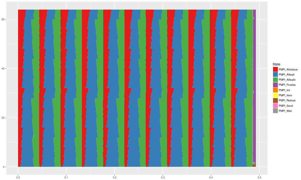
4.1. A Simple Gantt Chart
library(ggplot2)
df_state = read.csv("R_visualization/is_64.state.csv", header=F, strip.white=T)
names(df_state) = c("Type", "Rank", "Container", "Start", "End", "Duration", "Level", "State");
df_state = df_state[!(names(df_state) %in% c("Type","Container","Level"))]
df_state$Rank = as.numeric(gsub("rank-","",df_state$Rank))
head(df_state)
str(df_state)
  Rank    Start      End Duration          State
1    8 0.000000 0.000000 0.000000      PMPI_Init
2    8 0.000000 0.005703 0.005703 PMPI_Allreduce
3    8 0.005703 0.030164 0.024461  PMPI_Alltoall
4    8 0.030164 0.043736 0.013572 PMPI_Alltoallv
5    8 0.043736 0.049873 0.006137 PMPI_Allreduce
6    8 0.049873 0.074334 0.024461  PMPI_Alltoall
'data.frame':	2556 obs. of  5 variables:
 $ Rank    : num  8 8 8 8 8 8 8 8 8 8 ...
 $ Start   : num  0 0 0.0057 0.0302 0.0437 ...
 $ End     : num  0 0.0057 0.0302 0.0437 0.0499 ...
 $ Duration: num  0 0.0057 0.02446 0.01357 0.00614 ...
 $ State   : Factor w/ 9 levels "PMPI_Allreduce",..: 5 1 2 3 1 2 3 1 2 3 ...
gc = ggplot(data=df_state) +
   geom_rect(aes(xmin=Start, xmax=End, ymin=Rank, ymax=Rank+1,fill=State)) + scale_fill_brewer(palette="Set1")
gc
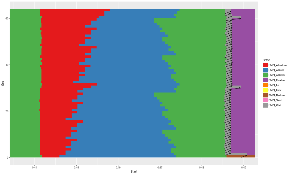
4.2. A Gantt Chart with Communications
df_link = read.csv("R_visualization/is_64.link.csv", header=F, strip.white=T)
names(df_link) = c("Type", "Level", "Container", "Start", "End", "Duration", "CommType", "Src", "Dst");
df_link = df_link[!(names(df_link) %in% c("Type","Container","Level","CommType"))]
df_link$Src = as.numeric(gsub("rank-","",df_link$Src))
df_link$Dst = as.numeric(gsub("rank-","",df_link$Dst))
head(df_link)
str(df_link)
     Start      End Duration Src Dst
1 0.485352 0.486841 0.001489  24  25
2 0.485431 0.486841 0.001410  25  26
3 0.485420 0.486842 0.001422   4   5
4 0.485480 0.486907 0.001427  61  62
5 0.485463 0.486914 0.001451  13  14
6 0.485504 0.486914 0.001410  14  15
'data.frame':	63 obs. of  5 variables:
 $ Start   : num  0.485 0.485 0.485 0.485 0.485 ...
 $ End     : num  0.487 0.487 0.487 0.487 0.487 ...
 $ Duration: num  0.00149 0.00141 0.00142 0.00143 0.00145 ...
 $ Src     : num  24 25 4 61 13 14 5 28 2 3 ...
 $ Dst     : num  25 26 5 62 14 15 6 29 3 4 ...
gc + geom_segment(data = df_link, aes(x = Start, y = Src, xend = End, yend = Dst),arrow = arrow(length = unit(0.01, "npc"))) +
   coord_cartesian(xlim = c(.9*min(df_link$Start), max(df_link$End)))
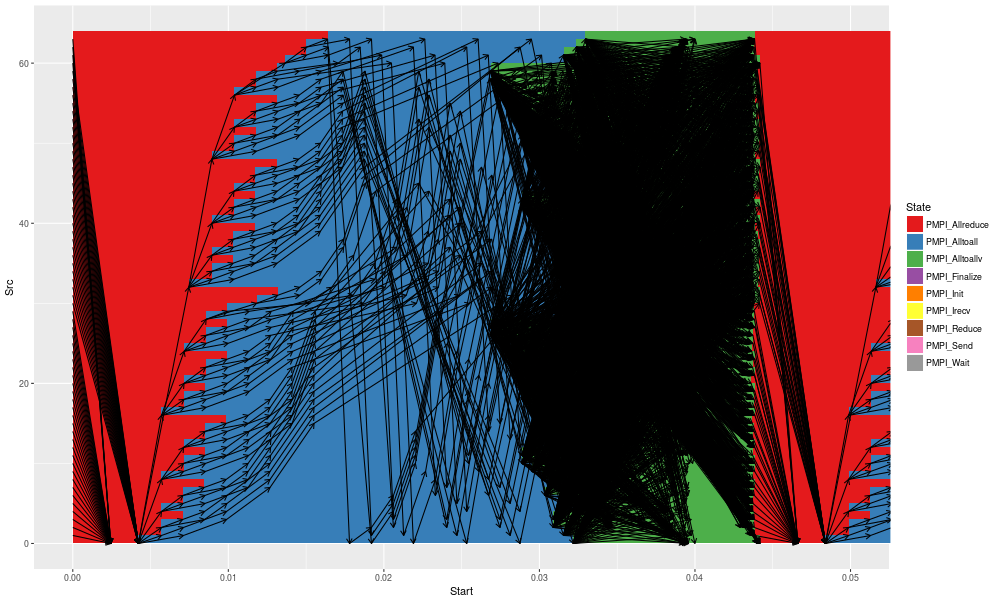
Unfortunately, the previous application mostly relies on collective communications so most MPI point-to-point communications do not show up. Fortunately, SimGrid allows you to trace such things (see the previous section), which allows to have a better undestanding of what happens:
df_link = read.csv("R_visualization/is_64_internal.link.csv", header=F, strip.white=T)
names(df_link) = c("Type", "Level", "Container", "Start", "End", "Duration", "CommType", "Src", "Dst");
df_link = df_link[!(names(df_link) %in% c("Type","Container","Level","CommType"))]
df_link$Src = as.numeric(gsub("rank-","",df_link$Src))
df_link$Dst = as.numeric(gsub("rank-","",df_link$Dst))
head(df_link)
str(df_link)
  Start      End Duration Src Dst
1 1e-06 0.002439 0.002438  61   0
2 1e-06 0.002439 0.002438   1   0
3 1e-06 0.002439 0.002438   2   0
4 1e-06 0.002439 0.002438   3   0
5 0e+00 0.002439 0.002439   4   0
6 0e+00 0.002439 0.002439   5   0
'data.frame':	49915 obs. of  5 variables:
 $ Start   : num  1e-06 1e-06 1e-06 1e-06 0e+00 0e+00 0e+00 0e+00 0e+00 0e+00 ...
 $ End     : num  0.00244 0.00244 0.00244 0.00244 0.00244 ...
 $ Duration: num  0.00244 0.00244 0.00244 0.00244 0.00244 ...
 $ Src     : num  61 1 2 3 4 5 6 7 8 9 ...
 $ Dst     : num  0 0 0 0 0 0 0 0 0 0 ...
gc + geom_segment(data = df_link, aes(x = Start, y = Src, xend = End, yend = Dst),arrow = arrow(length = unit(0.01, "npc"))) +
    coord_cartesian(xlim = c(0,.05))
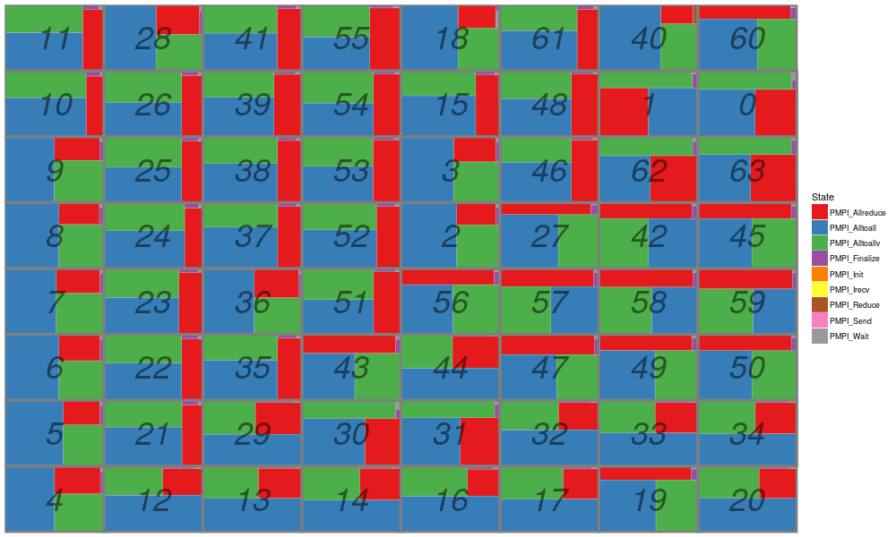
4.3. A Treemap
library("treemapify")
library("dplyr")
sessionInfo()
R version 3.4.2 (2017-09-28)
Platform: x86_64-pc-linux-gnu (64-bit)
Running under: Debian GNU/Linux 9 (stretch)

Matrix products: default
BLAS: /usr/lib/libblas/libblas.so.3.7.0
LAPACK: /usr/lib/lapack/liblapack.so.3.7.0

locale:
 [1] LC_CTYPE=fr_FR.UTF-8       LC_NUMERIC=C
 [3] LC_TIME=fr_FR.UTF-8        LC_COLLATE=fr_FR.UTF-8
 [5] LC_MONETARY=fr_FR.UTF-8    LC_MESSAGES=fr_FR.UTF-8
 [7] LC_PAPER=fr_FR.UTF-8       LC_NAME=C
 [9] LC_ADDRESS=C               LC_TELEPHONE=C
[11] LC_MEASUREMENT=fr_FR.UTF-8 LC_IDENTIFICATION=C

attached base packages:
[1] stats     graphics  grDevices utils     datasets  methods   base

other attached packages:
[1] treemapify_2.4.0 tidyr_0.7.2      dplyr_0.7.4      ggplot2_2.2.1

loaded via a namespace (and not attached):
 [1] Rcpp_0.12.13       digest_0.6.12      assertthat_0.2.0   grid_3.4.2
 [5] plyr_1.8.4         R6_2.2.2           gtable_0.2.0       magrittr_1.5
 [9] scales_0.5.0       rlang_0.1.4        lazyeval_0.2.1     bindrcpp_0.2
[13] labeling_0.3       RColorBrewer_1.1-2 glue_1.2.0         purrr_0.2.4
[17] munsell_0.4.3      compiler_3.4.2     pkgconfig_2.0.1    colorspace_1.3-2
[21] ggfittext_0.5.0    bindr_0.1          tibble_1.3.4
df_state %>% group_by(State,Rank) %>%
   summarise(Duration = sum(Duration)) %>%
   ggplot(aes(area = Duration, fill = State, subgroup = Rank)) + geom_treemap() +
   geom_treemap_subgroup_border() +
   geom_treemap_subgroup_text(place = "centre", grow = F, alpha = 0.5, colour =
                              "black", fontface = "italic", min.size = 0) +
   scale_fill_brewer(palette="Set1")
Aggregation at some level can be done with dplyr. We'll give some examples at some point but do not hesitate to as us if you don't know how to do so.
4.4. A Simple View Exploiting Resource Usage
df_var = read.csv("R_visualization/is_64_small.variable.csv", header=F, strip.white=T)
names(df_var) = c("Container", "Resource_Name", "Type", "Start", "End", "Duration", "Value");
df_var = df_var[!(names(df_var) %in% c("Container"))]
df_var = df_var %>% mutate(Resource_Name = as.character(Resource_Name))
head(df_var)
str(df_var)
  Resource_Name           Type    Start       End  Duration        Value
1             3        latency 0.000000 44.515197 44.515197 5.140000e-04
2             3 bandwidth_used 0.003752  0.009539  0.005787 5.027545e+05
3             3 bandwidth_used 0.009539  0.009540  0.000001 5.942425e+05
4             3 bandwidth_used 0.009540  0.014243  0.004703 5.517688e+05
5             3 bandwidth_used 0.014243  0.014386  0.000143 8.792511e+05
6             3 bandwidth_used 0.014386  0.029386  0.015000 0.000000e+00
'data.frame':	269141 obs. of  6 variables:
 $ Resource_Name: chr  "3" "3" "3" "3" ...
 $ Type         : Factor w/ 69 levels "bandwidth","bandwidth_used",..: 3 2 2 2 2 2 2 2 2 2 ...
 $ Start        : num  0 0.00375 0.00954 0.00954 0.01424 ...
 $ End          : num  44.5152 0.00954 0.00954 0.01424 0.01439 ...
 $ Duration     : num  4.45e+01 5.79e-03 1.00e-06 4.70e-03 1.43e-04 ...
 $ Value        : num  5.14e-04 5.03e+05 5.94e+05 5.52e+05 8.79e+05 ...
df_var %>% filter(Type == "bandwidth_used") %>% filter(Resource_Name != "loopback") %>%
    ggplot(aes(x=Start,y=Value)) + geom_step() + facet_wrap(~Resource_Name)
4.5. A network topology plot
Let's extract the topology:
df_topo = read.csv("R_visualization/is_64_small.link.csv", header=F, strip.white=T)
names(df_topo) = c("Type", "Level", "Container", "Start", "End", "Duration", "CommType", "Src", "Dst");
df_topo = df_topo[df_topo$CommType == "topology",];
df_topo = df_topo[(names(df_topo) %in% c("Container","Src","Dst"))]
head(df_topo)
str(df_topo)
      Container Src Dst
1 0-LINK8-LINK8   2   0
2 0-LINK8-LINK8   3   0
3 0-LINK8-LINK8   0   1
4 0-LINK8-LINK8  16  10
5 0-LINK8-LINK8   6  10
6 0-LINK8-LINK8  10  11
'data.frame':	46 obs. of  3 variables:
 $ Container: Factor w/ 4 levels "0-HOST3-LINK8",..: 3 3 3 3 3 3 3 3 3 3 ...
 $ Src      : Factor w/ 91 levels "0","1","10","11",..: 8 9 1 6 17 3 17 16 1 6 ...
 $ Dst      : Factor w/ 92 levels "0","1","10","11",..: 1 1 2 3 3 4 4 5 6 7 ...
library(dplyr)
library(ggplot2)
library(ggrepel)
#library(geomnet)
library(ggnetwork)
library(network)
sessionInfo()
network: Classes for Relational Data
Version 1.13.0 created on 2015-08-31.
copyright (c) 2005, Carter T. Butts, University of California-Irvine
                    Mark S. Handcock, University of California -- Los Angeles
                    David R. Hunter, Penn State University
                    Martina Morris, University of Washington
                    Skye Bender-deMoll, University of Washington
 For citation information, type citation("network").
 Type help("network-package") to get started.
R version 3.4.2 (2017-09-28)
Platform: x86_64-pc-linux-gnu (64-bit)
Running under: Debian GNU/Linux 9 (stretch)

Matrix products: default
BLAS: /usr/lib/libblas/libblas.so.3.7.0
LAPACK: /usr/lib/lapack/liblapack.so.3.7.0

locale:
 [1] LC_CTYPE=fr_FR.UTF-8       LC_NUMERIC=C
 [3] LC_TIME=fr_FR.UTF-8        LC_COLLATE=fr_FR.UTF-8
 [5] LC_MONETARY=fr_FR.UTF-8    LC_MESSAGES=fr_FR.UTF-8
 [7] LC_PAPER=fr_FR.UTF-8       LC_NAME=C
 [9] LC_ADDRESS=C               LC_TELEPHONE=C
[11] LC_MEASUREMENT=fr_FR.UTF-8 LC_IDENTIFICATION=C

attached base packages:
[1] stats     graphics  grDevices utils     datasets  methods   base

other attached packages:
[1] network_1.13.0   ggnetwork_0.5.1  ggrepel_0.7.0    bindrcpp_0.2
[5] treemapify_2.4.0 tidyr_0.7.2      dplyr_0.7.4      ggplot2_2.2.1

loaded via a namespace (and not attached):
 [1] Rcpp_0.12.13         bindr_0.1            magrittr_1.5
 [4] munsell_0.4.3        colorspace_1.3-2     R6_2.2.2
 [7] rlang_0.1.4          plyr_1.8.4           grid_3.4.2
[10] gtable_0.2.0         sna_2.4              lazyeval_0.2.1
[13] assertthat_0.2.0     digest_0.6.12        tibble_1.3.4
[16] purrr_0.2.4          RColorBrewer_1.1-2   ggfittext_0.5.0
[19] glue_1.2.0           statnet.common_4.0.0 labeling_0.3
[22] compiler_3.4.2       scales_0.5.0         pkgconfig_2.0.1
Here is a possible approach:
set.seed(57)
# Let's create the network
edgelist = df_topo[names(df_topo)[-1]]
edgelist$Src = as.character(edgelist$Src)
edgelist$Dst = as.character(edgelist$Dst)
n = network(x = edgelist)

# Let's obtain the nodes and their type (CPU vs. Link)
nodelist = data.frame(Label = unique(c(as.character(df_topo$Src),as.character(df_topo$Dst))))
nodelist$Label = as.character(nodelist$Label)
nodelist$Type = "Link"
nodelist[grepl("[a-z]",nodelist$Label),]$Type = "CPU"
# Let's reorder nodelist according to the network node list order
nodelist = nodelist[match(network.vertex.names(n),nodelist$Label,),]
set.vertex.attribute(n,"Type",nodelist$Type)
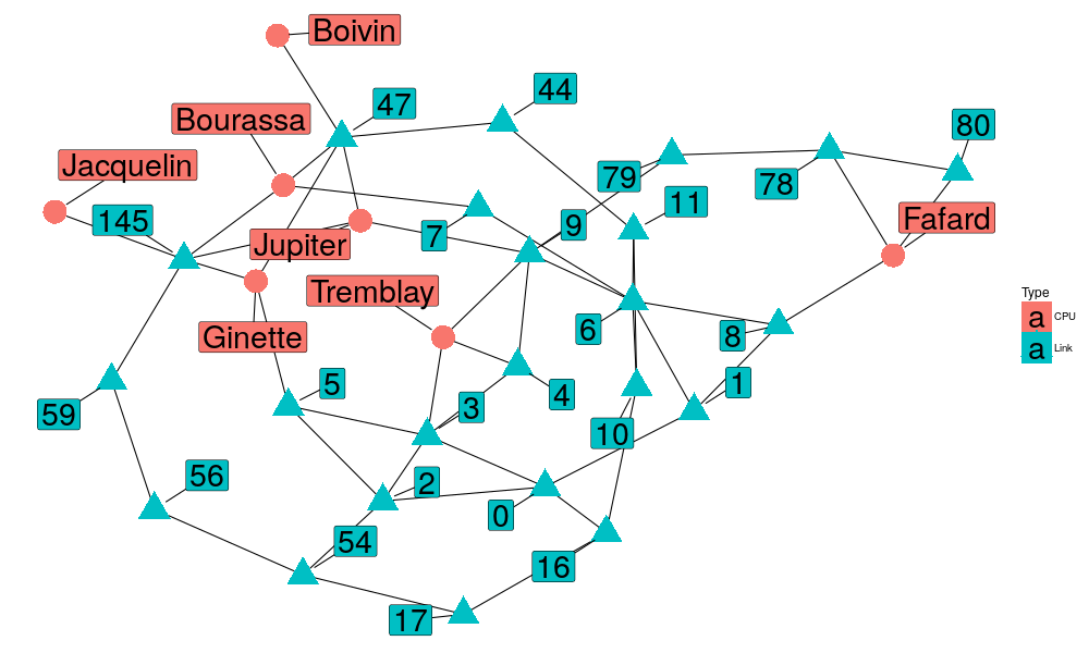
Then you could plot it through the ggnetwork
set.seed(72)
ggplot(n, aes(x, y, xend = xend, yend = yend)) +
       geom_edges(color = "steelblue") +
       geom_nodes(size = 10, aes(color = Type, shape = Type)) +
       geom_nodelabel_repel(aes(label = vertex.names),size=15) +
       theme_blank()
Or you could obtain these coordinates directly from the network package.
set.seed(57)
nlayout= network.layout.fruchtermanreingold(n, NULL)
nlayout= network.layout.kamadakawai(n, NULL)
nodelist$x=nlayout[,1]
nodelist$y=nlayout[,2]
# Let's propagate
edgelist = edgelist %>%
    left_join(nodelist[c("Label","x","y")],by = c("Src"="Label")) %>%
    rename(Src.x = x, Src.y =y ) %>%
    left_join(nodelist[c("Label","x","y")],by = c("Dst"="Label")) %>%
    rename(Dst.x = x, Dst.y =y )
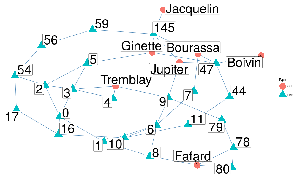
This allows us to have a better control on how things are plotted:
ggplot(nodelist, aes(x=x, y=y)) +
       geom_segment(data=edgelist, aes(x=Src.x, y=Src.y, xend=Dst.x, yend = Dst.y)) +
       geom_point(size = 10, aes(color = Type, shape = Type)) +
       geom_label_repel(aes(label=Label, fill=Type), size=10, segment.colour="black", box.padding = .5, point.padding = 1.5) +
       theme_blank()
Let's assume we have node values to account for (e.g., bandwidth, power, etc.):
df_var = df_var %>% left_join(nodelist %>% select(Label,Type) %>% rename(Resource_Type = Type), by=c("Resource_Name"="Label"))
Let's make a temporal aggregation (yeah, this one is a bit complicated but we wanted the end result to look nice…):
df_usage = df_var %>% # filter(Start <1) %>%
    group_by(Resource_Name, Resource_Type, Type) %>%
    summarise(value = sum(Value*Duration)) %>%
    filter(Resource_Name != "loopback", Type %in% c("power", "power_used", "bandwidth", "bandwidth_used")) %>%
    left_join(nodelist %>% select(-Type), by=c("Resource_Name"="Label")) %>% ungroup() %>%
    gather(key,value, -Resource_Name, -Resource_Type, -Type, -x, -y) %>%
    mutate(Type = case_when(
               Type == "bandwidth" ~ "capacity",
               Type == "power" ~ "capacity",
               Type == "bandwidth_used" ~ "utilization",
               Type == "power_used" ~ "utilization",
               TRUE ~ "<NA>")) %>% select(-key) %>% spread(Type, value) -> df_usage
df_usage
# A tibble: 30 x 6
   Resource_Name Resource_Type          x         y   capacity utilization
 *         <chr>         <chr>      <dbl>     <dbl>      <dbl>       <dbl>
 1             0          Link -1.3890409 -4.078463 1837548337   2649388.3
 2             1          Link -0.2496466 -3.312484 1526231307   1868998.2
 3            10          Link -0.6887878 -3.068336 1526231307   1011673.4
 4            11          Link -0.7127339 -1.499482 5283174690   1143084.2
 5           145          Link -4.1508398 -1.790682  114999447    993937.8
 6            16          Link -0.9209932 -4.539063 1526231307   1011673.4
 7            17          Link -2.0139672 -5.360228 5283174690    231283.3
 8             2          Link -2.6302089 -4.220480 5283174690   2250029.4
 9             3          Link -2.2902528 -3.562545 1526231307   2691311.2
10             4          Link -1.5980237 -2.863981  449586797   1529889.8
# ... with 20 more rows
Mmmh, unfortunately, on this example, utilization is ridiculously
small compared to capacity. :( Let's create fake values for the sake
of the visualization but at least, you know how to extract data from
the trace and process it…
df_usage$capacity = runif(length(df_usage$Resource_Name))
df_usage$utilization = runif(length(df_usage$Resource_Name))*df_usage$capacity
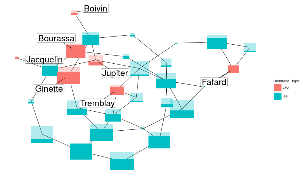
Let's create a specific geom_ to draw the boxes for us.
geom_simgrid_node = function(d) {
    xr = .7
    d %>% mutate(utilization = utilization/capacity) %>%
        mutate(capacity = capacity/max(capacity)) -> d
    d$xmin = d$x - xr*sqrt(d$capacity)/2
    d$xmax = d$x + xr*sqrt(d$capacity)/2
    d$ymin = d$y - xr*sqrt(d$capacity)/2
    d$ymax = d$y + xr*sqrt(d$capacity)/2
    d$ymax_fill = d$ymin + d$utilization *  (d$ymax - d$ymin) # d$utilization * xr*sqrt(d$capacity)
    ret = list(
       geom_rect(data=d,size = 10, aes(xmin=xmin, xmax=xmax, ymin=ymin, ymax=ymax, fill = Resource_Type),alpha=.3),
       geom_rect(data=d,size = 10, aes(xmin=xmin, xmax=xmax, ymin=ymin, ymax=ymax_fill, fill = Resource_Type)))
    return(ret)
}
Now, links are in blue, hosts in red, the size of the rectangles is proportional to their capacity and the darker area inside is proportional to their average use.
set.seed(54)
ggplot(df_usage, aes(x=x, y=y)) +
       geom_segment(data=edgelist, aes(x=Src.x, y=Src.y, xend=Dst.x, yend = Dst.y)) +
       geom_simgrid_node(df_usage) +
       geom_label_repel(data=df_usage[df_usage$Resource_Type=="CPU",],
                        aes(label=Resource_Name), size=10, segment.colour="black",
                        box.padding = .5, point.padding = 1.5) +
       theme_blank()
4.6. TODO Jedule / SimDAG view


